Organic and Elemental Carbon in Atmospheric Fine Particulate Matter in an Animal Agriculture Intensive Area in North Carolina: Estimation of Secondary Organic Carbon Concentrations ()
1. Introduction
Particulate matter (PM) contains a significant fraction of carbonaceous materials. The carbonaceous materials are usually classified as elemental carbon (EC) and organic carbon (OC) [1]. Elemental carbon generates predominantly from incomplete combustion process, and it has been used as a tracer for primary OC (POC) [2]. Organic carbon includes POC, which refers to carbon material emitted in particulate form, and secondary OC (SOC), which is formed through atmosphere physical and chemical reactions [1]. Carbon-containing components (EC and OC) occupy very important fractions of PM, and they account typically 10% to 50% of atmospheric PM mass [1,3]. Although knowledge about POC and SOC is important to develop strategies for controlling particulate carbon pollution, quantification has been difficult to accomplish because of the complexity and no simple analytical methods available. Several methods have been applied to estimate the fraction of SOC [2,4-9]. The thermographic analysis method, which is performed on PM samples collected on quartz filters, can classify organic compounds into groups [7,8]. In this method, a carbon thermogram may be constructed by plotting the evolved carbon as a function of temperature. The thermogram peaks can then be used for source allocation, i.e., primary and secondary portions of carbon-containing component studies [5,8]. Hildemann, et al. [6] used carbon isotopic composition (14C/12C) to estimate the SOC in the Los Angeles basin. Turpin, et al. [2,9] applied OC/EC ratios to quantify the presence of SOC. Castro, et al. [4] estimated SOC using the minimum ratio of OC/ EC. The OC/EC primary ratio analysis is an acceptable method for SOC estimation.
In the United States (US) the Clean Air Act (CAA) was signed into law in 1970 and the US environmental protection agency (EPA) established the national ambient air quality standards (NAAQS) to protect public health and environment under the CAA. To assess national ambient air quality and implement NAAQS, the EPA has established a comprehensive ambient air monitoring program, which has been carried out by state and local agencies [11]. All the EPA monitoring networks have provided numerous high quality datasets for air quality and public health studies. However, these existing networks do not provide enough representative scientific data for assessment of ambient air quality in rural areas, especially in agricultural intensive areas.
As of the most recent Agricultural Census [12], North Carolina (NC) ranked second in the nation in the production of hog and poultry. Because of the rapid growth of swine and poultry industry, significant increases of ambient air pollutant concentrations (e.g. NH3) were observed in NC coastal plain regions [13,14]. Regional intensive agricultural activities (especially livestock and poultry industry) pose substantial risks to air quality and public health. Quantitative information concerning the presence of SOC is still scarce, and to the authors’ knowledge, there is no publication addressing this subject quantitatively in animal agriculture intensive areas.
In this study, a field investigation was conducted to characterize the OC and EC of PM2.5 inside and in the immediate vicinity of a large commercial egg production farm. The objectives were to: 1) provide an OC/EC dataset for animal agriculture intensive areas; 2) present OC thermal characterization information; 3) assess POC and SOC in order to understand the contribution of SOC to the total organic carbon (TOC) in PM2.5.
2. Methodology
2.1. The Research Site and Field Sampling Locations
The field sampling of PM2.5 was conducted in an animal agriculture intensive area in NC. As shown in Figure 1, samples of PM2.5 were simultaneously taken at five stations: an emission source (a high rise egg production house: ST1), and the ambient stations (ST2-5) surrounding the farm nearby the property lines of the egg production farm. The filed sampling campaign covered four seasons from December 2008-December 2009 and 312 samples were taken. While the data series were not continuous, the numbers of samples were sufficient to give a very good representation of the variability of the concentrations over the sampling periods.
Sampling was performed with Partisol (Model 2300) chemical speciation samplers, operated for durations ranging from 8 to 24 hours. Three cartridges with different filters (Nylon, Teflon and Quartz) were used to collect PM2.5 samples. Nylon filter was used for ion analyses [15,16], Teflon filter was used for trace element and mass analyses [17], and Quartz filter was used for organic and element carbon analyses. Each cartridge contains a sharp-cut PM2.5 impactor operating at a flow rate of 10.0 L/min (nylon and quartz) or 16.7 L/min (Teflon). Filters were kept and transported to field in individual petri dishes. After sampling, exposed filters were stored at 4˚C and transported to the analysis laboratory.
2.2. Thermal-Optical Aerosol Analyzer: Carbon Analyses
The collected quartz filters were analyzed for OC/EC at RTI aerosol laboratory (RTP, NC, US) using a ThermalOptical Carbon Aerosol Analyzer (Sunset Laboratory Inc., OR, USA). Figure 2 shows the schematic diagram of the analyzer. A punch of subsample from a quartz filter was placed in a quartz boat of the analyzer and the light diode laser was used to monitor transmittance of the filter during analysis. A thermocouple was, used to monitor sample temperature during analysis. The front oven

Figure 1. The layer farm layout and the PM2.5 sampling stations [10].

Figure 2. Schematic diagram of a thermal-optical carbon analyzer.
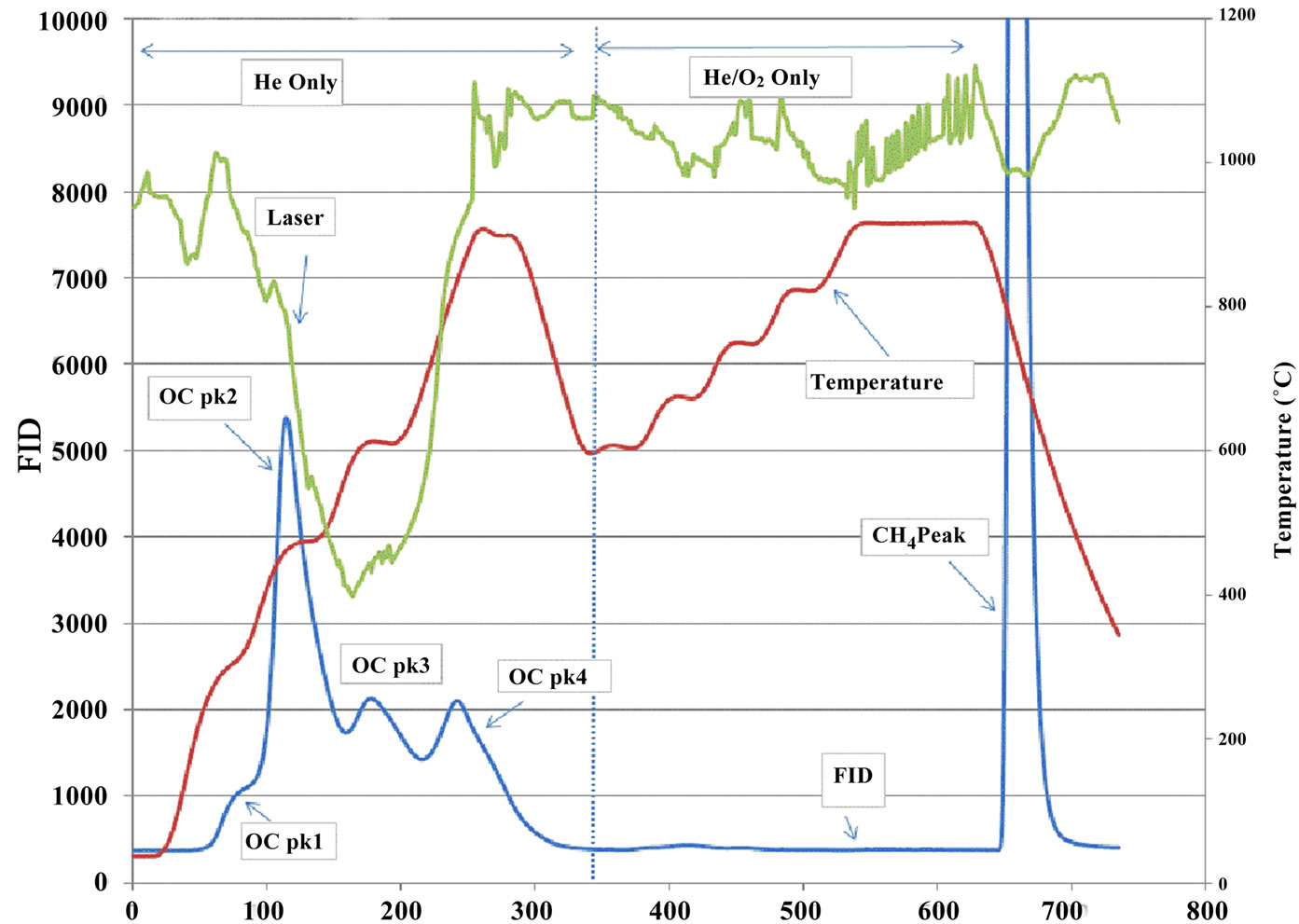
heating program was the NIOSH-like method used as part of the PM2.5 Speciation Trends Network [18]. The NIOSH method started with a 10-sec purge, followed by four 60-sec temperature ramps (310˚C, 480˚C, 615˚C and 900˚C) in a non-oxidizing atmosphere (Helium), then after cooling oven to 600˚C, a series of 45-sec four heating ramps (600˚C, 675˚C, 750˚C, 825˚C) and 120-sec at 920˚C was applied in a 2% oxygen in helium atmosphere (Figure 3). All carbon species evolved from the filter are converted to carbon dioxide (CO2) in oxidizer oven (870˚C), and CO2 is reduced to methane and detected using a flame ionization detector (FID). OC Pk1, OC Pk2, OC Pk3 and OC Pk4 were the integration of the FID signal under four 60-sec temperature ramps in Helium atmosphere (Figure 3). Total OC is the summation of OC Pk1, OC Pk2, OC Pk2, OC Pk4 and pyrolysed OC. Peaks integrated at 2% O2/98% He atmosphere and subtracted pyrolysed OC were EC. The optical measurement was used to correct for pyrolysis or charring of OC during heating process. This method reports only carbon contents and does not directly account for the mass of hydrogen, oxygen and any other elements.
2.3. Estimations of SOC Concentrations Using the Minimum Value of OC/EC Ratio Method
At this research site, there were evidences of the influence of SOC that were transported or formed in this agriculture intensive sampling area. Since no experimenttal method could be used to directly measure SOC fraction, Turpin and Huntzicker [2] proposed using EC and OC data to estimate the SOC fraction. Elemental carbon, emitted mainly by combustion sources, was used as a tracer of primary fraction of OC. In the proposed method, for a given site, the OC-to-EC ratio ((OC/EC)pri), representative of the primary emissions of EC and OC, was assumed to be relative constant and do not evolve significantly.
The concentration of SOC can then be calculated from the equation:
 (1)
(1)
where, OCtotal is the total OC, the summation of OC Pk1, OC Pk2, OC Pk2, OC Pk4 and pyrolysed OC.
Statistical analyses were performed using SAS/STAT software, version 9.2 (SAS Institute Inc., Cary, NC, USA). The paired t-test analyses were performed to test the statistical differences between different stations. Multivariate analyses were conducted to elucidate possible relationship among them. A factor analysis was conducted for the correlation matrix of the variable analyzed, using principle component analysis as the extraction methods. The rotation method of VARIMAX was used. Variable standardization was performed in order to have means of zeros and variances of one.
3. Results and Discussion
3.1. Overall Means of Samples from In-House and Ambient Stations
The overall mean concentrations of PM2.5 mass, OC, EC, and total carbon (TC, the summation of OC and EC) are given in Table 1, which also includes the numbers of samples, standard deviations (Std.), medians, minimums and maximums. In poultry house (ST1), the average OC and EC concentrations were higher than ambient stations. The high OC concentrations at ST1 indicated that most of PM2.5 was contributed by organic matter (e.g., crude feed protein, crude feed fiber, and animal dander) generated from mechanical processes. In the poultry house, there was no bio-based fuel heating system, so there was very little EC generated in the poultry houses. The reported EC at ST1 might be due to the uncertainty from the pyrolysis correction [29]. At ambient stations (ST2-5), OC concentrations were slightly higher than 3.0 µg/m³, and EC concentrations were about 10% of OC. The average OC and EC levels for ambient stations were within the range given by other studies at other regional rural or background sites (Table 2). The OC to PM2.5 mass ratios (36% - 40%) were higher than most values reported in the literature. The possible reasons may be due to the
 (a)
(a)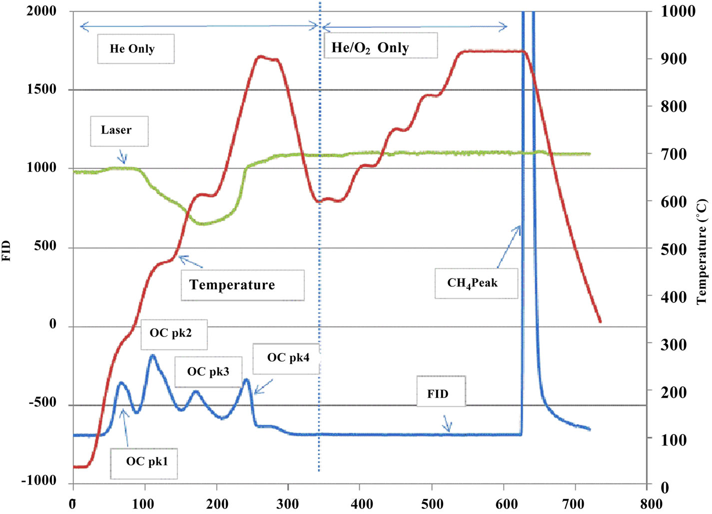 (b)
(b)
Figure 3. Typical thermograms. (a) a sample from the in house station; (b) a sample from an ambient station.
fact that this research site was in a rural agriculture area with a large egg production facility. Local agriculture activities might result in different OC to PM2.5 ratios from other areas if the farming practices are different. Turpin and Huntzicker [9] and Chow, Watson [20] used the ratios of OC to TC concentrations to study emission and transformation characteristics of carbonaceous species in particulate. As it is well known, EC originates primarily from direct emissions, whereas OC can originnate from direct emissions and atmospheric transformations. The average ratios of OC/TC were similar at four ambient stations (Table 1), and these ratios were higher than the reported values [20]. The distribution of OC/TC ratios from all ambient sites is shown in Figure 4. The OC/TC ratio were greater than most of the OC/TC ratio of the primary aerosol (emissions by different sources), which indicated secondary formation occurred [2,21]. The high OC/TC ratios at the ambient stations were pos-


Table 1. Descriptive statistics of mass concentration, OC, and EC of PM2.5 samples.

Table 2. Elemental and organic carbon levels found in PM2.5 from different regions of the world.

Figure 4. The distribution of OC/TC ratios at ambient stations.
sible due to biogenic emissions, anthropogenic emissions, and atmospheric transport and transformation. Forest fire, natural gas home appliances, meat charbroiling, etc. might also result in high OC/TC ratio [21].
By checking into the relationship between OC and EC, the relative importance of biogenic and anthropogenic emissions of OC and transport can be examined [22]. If there was strong correlation between OC and EC, it was likely that they were transported simultaneously from other regions or emitted from a similar source.
The relationships between OC and EC concentrations at ambient stations (ST2-5) are shown in Figure 5. The observed weak relationships between OC and EC (correlation coefficients r < 0.1) suggested that OC and EC of PM2.5 at this research site were not transported simultaneously from other regions, and the local biogenic and anthropogenic OC emissions were very important.
3.2. Thermograms
Figure 3 illustrates the distinctions between samples collected in house and at ambient stations. The marked peaks of OC Pk1, OC Pk2, OC Pk3, OC Pk4, pyrolysed OC and EC are the principal features of the thermograms. The OC Pk1 observed approximately 310˚C corresponds to the volatilization of lower molecular weight organics. The OC Pk2, OC Pk3, and OC Pk4 at approxi-