Transient Waves Due to Thermal Sources in a Generalized Piezothermoelastic Half-Space ()
1. Introduction
Application of different types of loads on the surface of piezoelectric materials is an active research subject for engineers and scientists. Smart and intelligent structures are developed to enhance the performance of the structural components. In some cases, the load bearing substrates of these smart structures are made of composite materials. Ashida et al. [1] provides an overview of the use of piezoelectric materials in intelligent structures for aerospace applications. The mechanical and fracture properties of piezoelectric ceramics under thermal loading conditions have gained much attention [2,3]. There are some factors such as economical, less fuel consumption, higher speed achievement, ability to adapt to various applied loads and environment, which increases the interest to enhance the performance (e.g. load carrying capacity, crash or buckling behaviors) of the structural components in aerospace, ground vehicles, hydrospace, nuclear engineering, navigation, civil, mechanical engineering and ship manufacturing industries etc.
The theory of coupling of thermal and strain fields gives rise to coupled thermoelasticity and was formulated by Duhamel [4], which predicts the infinite speed of heat transportation. Lord and Schulman [5] and Green and Lindsay [6] have formulated non-classical (generalized) theories of thermoelasticity which eliminate the paradox of infinite velocity of heat propagation inherited in classical theory of thermoelasticity. According to these theories, heat propagation should be viewed as a wave phenomenon rather than diffusion one. A wave-like thermal disturbance is referred to as “second sound” by Chandrasekharaiah [7]. Ackerman et al. [8] and Ackerman and Overtone [9] proved experimentally for solid Helium that thermal waves (second sound) propagating with a finite, though quite large speed also exit. Guyer and Krumhansl [10] studied the second sound effect in solid Helium analytically. The recent and relevant theoretical development on this subject are due to Green and Nagdhi [11-13], which provide sufficient basic modification in the constitutive equations that permit treatment of a much wider class of heat flow problem.
Harinath [14,15] considered the problem of surface point and line source over a homogeneous isotropic generalized thermoelastic halfspace. Majhi [16] introduced a potential function and applied the LS theory to study the transient thermal response of a semi-infinite piezoelectric rod subjected to a local heat source along the length direction. The physical laws for the thermo-piezoelectric materials have been explored by Nowacki [17,18]. Chandrasekhariah [19,20] developed the generalized theory of thermo-piezoelectricity by taking in account the finite speed of propagation of thermal disturbances. Honig and Dhaliwal [21], solved a boundary value problem of an isotropic elastic halfspace with its plane boundary either rigidly fixed or stress free and subjected to sudden temperature increase. Nirula and Noda [22,23] treated the problems of crack breaking at the surface of piezothermoelastic semi-infinite body and a strip under steady thermal load. Sharma and Kumar [24] investigated the plane strain problems of transversely isotropic thermoelastic medium by employing an eigenvalue approach after applying the technique of Laplace and Fourier transform. Sharma et al. [25] studied the disturbances in the piezothermoelastic halfspace due to periodic strip thermal sources acting on its surface. The model of two dimensional equations of generalized magneto-thermoelasticity in a perfectly conducting medium has been established by Aouadi [26].
The present paper deals with the distribution of temperature change, stresses and electric potential in a generalized piezo-thermoelastic (6 mm class) material halfspace due to impact and continuous strip thermal sources acting on its surface. A combination of the Laplace and Fourier integral transforms has been used to solve the problem in the transform domain. The results in the physical domain are attained with the help of a numerical technique for inverting the integral transforms [27]. The computer simulated results in respect of stresses; temperature change and electric potential have been presented graphically for cadmium selenide (6 mm class) material. A comprehensive analysis and comparison of results in various theories has been presented.
2. Formulation of the Problem
We consider a homogeneous, transversely isotropic, thermally conducting generalized piezothermoelastic halfspace which is initially at uniform temperature . We take
 axis along the poling direction and also as sume that the medium is transversely isotropic in the sense that the planes of isotropy are perpendicular to the
  axis. We take origin of the co-ordinate system
  at any point on the plane surface and
  axis pointing vertically downward into the halfspace, which is thus represented by
 . It is assumed that an impact/continuous strip thermal source is acting at the rigidly fixed surface
  of the medium as shown in the Figure 1. From the symmetry consideration all the field quantities are independent of
  coordinate. We further assume that the field quantities vanish as
  . Let
. Let ,
,  and
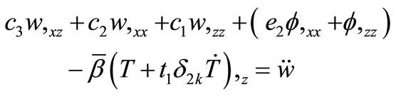
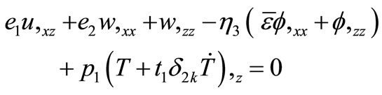
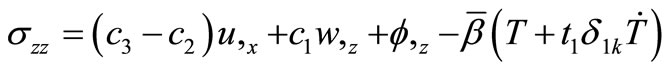
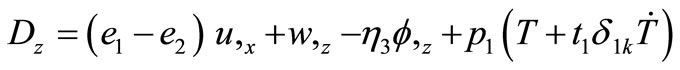
and  respectively, denote displacement vector, temperature change and electric potential in the considered solid. The non-dimensional basic governing field equations and constitutive relations for a homogeneous, transversely isotropic piezothermoelastic solid halfspace; in the absence of charge density, heat sources and body forces, are given by Sharma and Walia [28].
 (1)
(1)
 (2)
(2)
 (3)
(3)
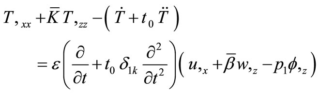 (4)
(4)
 (5)
(5)
 (6)
(6)
 (7)
(7)
 (8)
(8)
 and
and  are the electrical displacement and electric potential, respectively. The superposed dot denotes time
derivatives and coma notation is used for spatial derivatives.
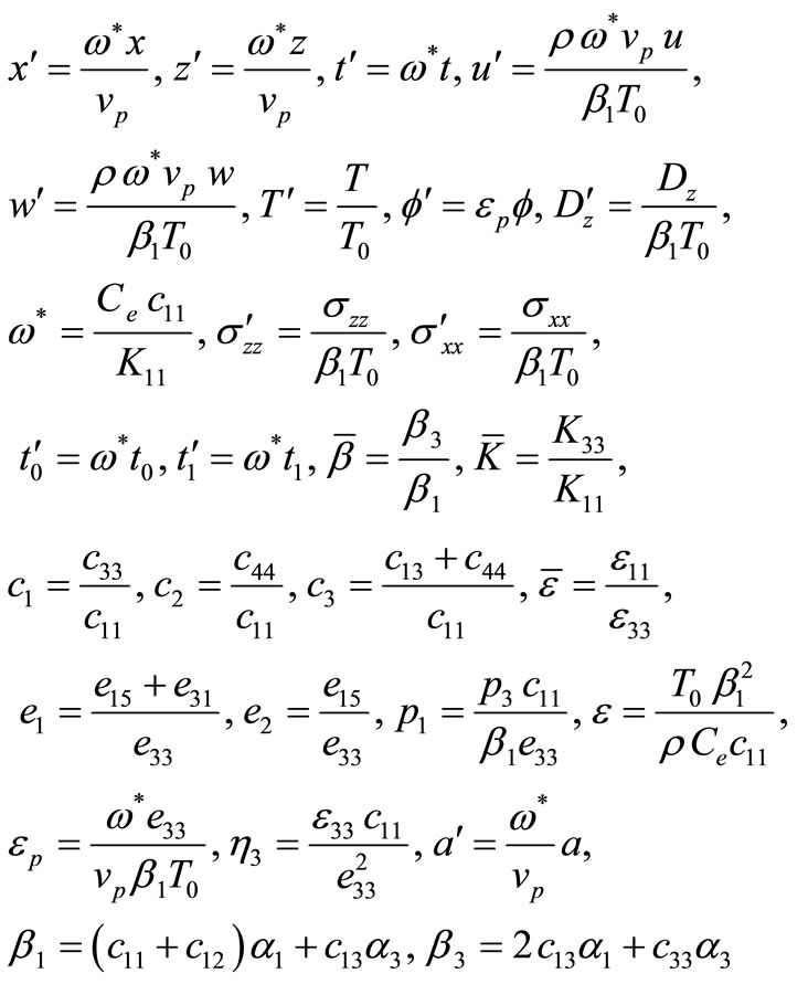
Where we have defined and used the quantities
 (9)
(9)
The primes have been suppressed for convenience. Here ,
,  and
and ,
,  are respectively, the coefficients of linear thermal expansion and thermal conductivity, in the direction orthogonal to the axis of symmetry and along the axis of symmetry;
  and
and  are the mass density and specific heat at constant strain, respectively;
  is the thermoelastic coupling constant;
  is the characteristic frequency of the medium;
  is piezothermoelastic coupling constant;
  are elastic parameters;
  are piezoelectric constants;
 ,
,  are the electric permittivities perpendicular and along the axis of symmetry;
  is pyroelectric constant in
  direction;
  and
and  are respectively denote stresses and electrical displacement;
 ,
,  are the thermal relaxation time parameters and
  is the longitudinal wave velocity in the medium. The symbol
 is Kronecker’s delta in which
  corresponds to the Lord-Shulman (LS) and
  refers to the Green-Lindsay (GL) theories of thermoelasticity. The thermal relaxation time parameters
  and
and  satisfy the inequalities
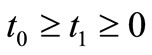 (10)
(10)
in case of GL theory only. However, it has been proved by Strunin [29] that the Inequalities (10) are not necessary to be satisfied.
3. Initial, Regularity and Boundary Conditions
The following initial and regularity conditions are assumed to be satisfied:
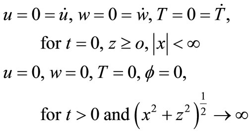 (11)
(11)
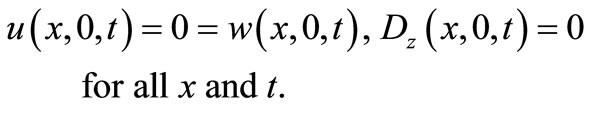
In addition to above boundary conditions, the surface  of the piezothermoelastic solid is subjected to time dependant strip thermal sources (impact or continuous) in the region
  and assumed to be rigidly fixed and charge free (open circuit). Therefore, the corresponding boundary conditions are given as Rigidly fixed and open circuit:
 (12.1)
Temperature input (TI):
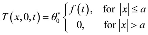 (12.2)
Temperature gradient (TG):
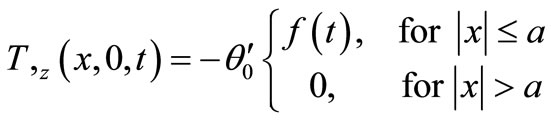 (12.3)
where ,
,  and
and , the prime has been suppressed. Here the function
  is a well behaved function of time and is defined as
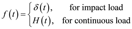
where  is a Heaviside unit step function,
  denotes the Dirac delta function.
4. Solution of the Problem
In order to solve the problem we apply Laplace transform with respect to time ‘t’ and Fourier transform with respect to x defined by Churchill [30]
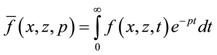 (13)
(13)
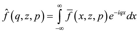 (14)
(14)
Upon operating Transformations (13) and (14) on the system of Equations (1) to (4), we obtain
 (15)
(15)
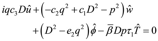 (16)
(16)
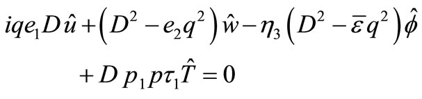 (17)
(17)
 (18)
(18)
where ,
, ,
, ,
, 
The above coupled system of ordinary differential Equations (15-18) upon retaining that part of the solution which satisfies the radiation condition  (j = 1, 2, 3, 4) leads to the following formal transformed solution
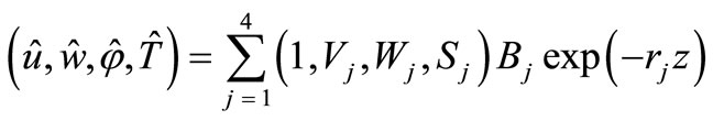 (19)
(19)
where ,
,  and
and  are the amplitude ratios, obtained as
 ,
,  ,
, (20)
(20)
and the characteristic roots  are given by the relations
 (21)
(21)
Here the quantities F,  and
and ,
,  are defined in the Appendix. Upon using Solution (19) in the Equations (5-8), the transformed stresses
  and electric displacement
  are obtained as
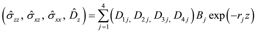 (22)
(22)
where
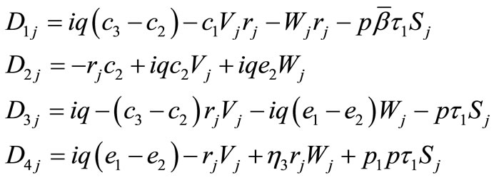 (23)
(23)
Upon applying integral transforms (13) and (14) to the boundary conditions (12) and using the Solution (22), we obtain a nonhomogeneous system of linear algebraic equations in the unknowns  for each set of conditions, TI or TG.
After solving the above system of equations we obtain
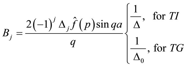 (24)
(24)
where 
 (25)
(25)
and  can be written from
  by replacing the permutation of suffixes (2, 3, 4) in
  and
and  with (1, 3, 4), (1, 2, 4) and (1, 2, 3) respectively.
Thus the transformed solutions of various field functions such as displacements, temperature change, stresses, electric potential and electric displacement can be obtained from Equations (19) and (22) upon solving the values of  from Equation (24) in case of thermal loads (TI/TG) under the considered electrical and mechanical conditions prevailing at the surface of the halfspace.
5. Inversion of the Transforms
Due to the existence of damping term in Equations (1-4) the dependence of characteristic roots 
 on the integral transform parameters
  and
and  is complicated. Hence analytically inversion of integral transform is difficult and cumbersome because the isolation of
  and q is not easily possible. This difficulty, however, can be overcome if we use some approximate or numerical methods. Therefore, in order to obtain the solution of the instant problem in the physical domain, we invert the integral transforms in Equations (19) and (22) by using a numerical technique [27] outlined below.
The expressions for various transformed field functions can formally be expressed as a function of ,
,  and
and  of the form
 . Upon inverting the Fourier transform, we get
 (26)
(26)
where  and
and  respectively, denote the even and odd parts of the function
  with respect to
 . For fixed values of
 ,
,  and
and , the function inside the braces in Equation (26) can be considered as a Laplace transform
  of some function
 . Using the inversion formula for Laplace transform [31] provides
 (27)
(27)
where  is an arbitrary real number greater than the real parts of the singularities of
 . Taking
 , the above Integral (27) takes the form
 (28)
(28)
Expanding the function  in Fourier series in the interval
 , the approximate Formula (28) becomes
 (29)
(29)
where
 (30)
(30)
 is the discretisation error which can be made arbitrarily small by choosing
  large enough. Since the infinite series in Equation (29) can be summed up to a finite number (N) of terms, the approximate value of h (t) becomes
 (31)
(31)
While using Formula (31) to evaluate , we also introduce a truncation error
  that must be added to the discretisation error to produce the total approximation error. In order to accelerate the process of convergence of the solution, the “Korrecktur” method is used to reduce the discretisation error and the
  algorithm is employed to reduce the truncation error. The Korrecktur formula provides us
  where
where  and
and . Thus, the approximate value of
  becomes
 (32)
(32)
where  is an integer such that
 . We shall now describe the
  algorithm that is used to accelerate the convergence of the series in Equation (31). Let N be an odd natural number and let
  be the sequence of partial sums of Equation (31). We define the
  sequence by
 ,
,  ,
, ;
; 
It can be shown that the sequence  converges to
  faster than the sequence of partial sums
  (m = 1, 2, 3,
 ). The actual procedure used to invert the Laplace transforms consists of using Equation (29) together with the
  -algorithm. The values of
  and
and  are chosen according to the criteria outlined by Honig and Hirdes [32].
The last step in the inversion process is to evaluate the Integral (26). According to Bradie [33], the various quadrature formulae such as Newton-Cotes, Romberg and Gaussian quadrature etc. can be used to approximate the value of an improper integral, provided the integral exists. However, some change of variable generally must be made to achieve theoretical order of convergence, if required. Here the evaluation of Integral (26) has been done by using Romberg integration with adaptive step size, which uses the results from successive refinements of the extended trapezoidal rule followed by extrapolation of the results to the limit when the step size tends to zero. The details can be found in Press et al. [34].
6. Numerical Results and Discussion
In order to illustrate and compare the theoretical results obtained in the previous sections, in the context of LS, GL and CT theories of thermoelasticity, we now present some numerical results. The material for the purpose of numerical calculations is taken as cadmium selenide (CdSe) having hexagonal symmetry (6 mm class) and belongs to the class of transversely isotropic material. The physical data for a single crystal of CdSe material is given below [28].
 ,
,  ,
,  ,
,  ,
,  ,
,  ,
,  ,
,  ,
,  ,
,  ,
,  ,
,  ,
,  ,
,  ,
,  ,
,  ,
,  ,
,  ,
,  ,
,  ,
,  ,
,  ,
,  ,
, 
The value of thermal relaxation time parameter  has been estimated from the relation
 , see Chandrasekharaiah [7]. We have taken
  for computation purpose. The computations are carried out for single value of time
  at
at . The complex characteristic equation formed by the Relations (21), being, in general of the form
 , can be solved for ‘r’ with the help of DesCartes procedure [27] along with irreducible case of Cardano’s method for fixed values of p and q. These are used to obtain temperature change (T), normal stress
 , shear stress
  and electric potential
  in the relevant relations. The numerical technique outlined in the Section 5 has been used to invert the Laplace and Fourier transforms. A FORTRAN code is developed and executed to compute various considered field functions due to two different types of strip thermal loads namely, temperature input (TI) and temperature gradient (TG) acting at the rigidly fixed, open circuit (OC) boundary of the piezothermoelastic halfspace. These computer simulated quantities are plotted in the Figures 2 to 9. The curves without ball, with solid ball and hollow ball correspond to LS, GL and CT theories of thermoelasticity, respecttively. The variations of temperature change (T), normal stress
 , shear stress
 , and electric potential
  with respect to epicentral distance
  due to strip of impact or continuous temperature input (TI) has been presented in the Figures 2 to 5 and due to temperature gradient (TG) in the Figures 6 to 9 on linear scales in the context of LS, CT and GL theories of thermoelasticity.
Figure 2 reveals that the profiles of temperature change  due to continuous or impact temperature input (TI) have maximum value in the vicinity of the load. The temperature change start decreasing with increasing epicentral distance and ultimately die out at certain values of epicentral distance
 , which ascertain

Figure 2. Variation of temperature change with epicentral distance due to continuous and impact temperature input.
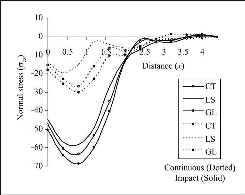
Figure 3. Variation of normal stress with epicentral distance due to continuous and impact temperature input.
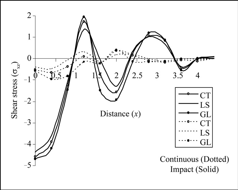
Figure 4. Variation of shear stress with epicentral distance due to continuous and impact temperature input.
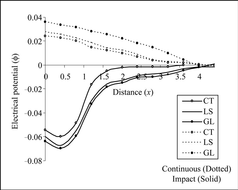
Figure 5. Variation of electric potential with epicentral distance due to continuous and impact temperature input.

Figure 6. Variation of temperature change with epicentral distance due to continuous and impact temperature gradient.
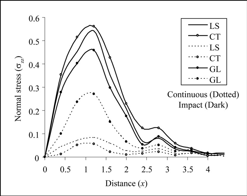
Figure 7. Variation of normal stress with epicentral distance due to continuous and impact temperature gradient.
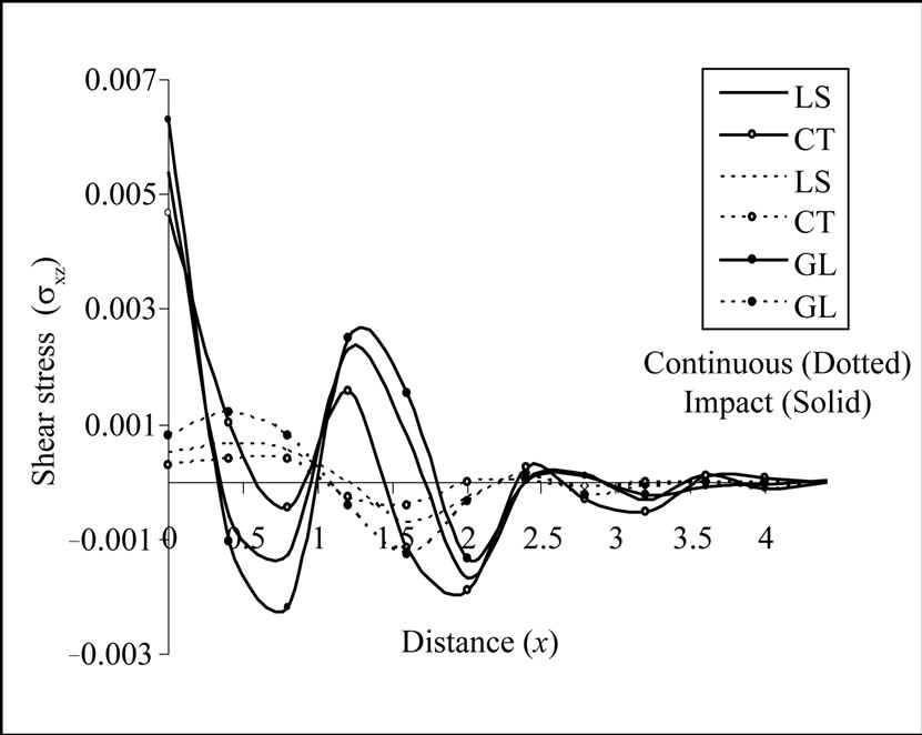
Figure 8. Variation of shear stress with epicentral distance due to continuous and impact temperature gradient.
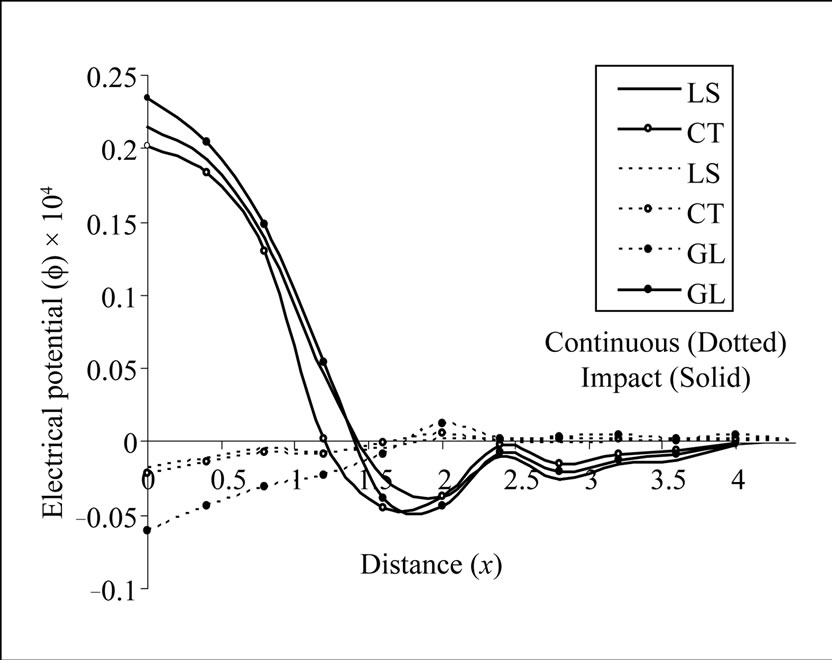
Figure 9. Variation of electrical potential with epicentral distance due to continuous and impact temperature gradient.
the existence of wave-front and finite speed of heat propagation. It is also revealed that the magnitude of temperature change  due to impact TI is signifycantly large as compared to that for continuous one. The various curves are quite distinguishable due to significant effect of thermal relaxation time. It is also observed that temperature change has a non-zero value only in a particular region of the halfspace and outside that region its values almost vanish identically which means that no thermal disturbance can be felt outside that particular region. On comparing the results of temperature change for three different theories of thermoelasticity, it is observed that
  for both impact and continuous load.
It is observed from Figure 3 that magnitude of normal stress  increases initially, attains maximum value and then decreases slowly to ultimately become asymptotically close to zero for
 , which again conforms the existence of wave fronts. This phenomenon is attributed to compression and expansion of the molecules of the solid due to application of the load. Initially, the internal friction due to application of temperature input at OC boundary increases which results in increase in the magnitude of normal stress followed by a rapid decay in the magnitude of normal stress due to decrease of internal friction. It is also observed that profiles of normal stress
  are clearly distinguishable due to signifycant effect of thermal relaxation times. The normal stress for three different theories of thermoelasticity follows the trend
  for both impact and continuous load.
Figure 4 shows the variation of shear stress  with epicentral distance
  in the context of GL, LS and CT theories of thermoelasticity. It is observed that shear stress
  devolvement due to continuous TI is comparatively small to that of impact temperature input (TI). The amplitude of vibrations gets suppressed due to increase in the internal friction among the molecules of the solid as we move away from vicinity of the load. Shear stress
  dies out in an oscillating fashion as we move away from vicinity of the load. However, the shear stress devolvement is very small as compared to the vertical stress
  which is consistent with the boundary conditions. Shear stress shows the trend
  for
for  in case of continuous load.
Figure 5 represents the variations of electric potential  with epicentral distance
 due continuous or impact temperature input (TI) acting on the OC boundary of the halfspace. Its magnitude is noticed to be signifycantly large near the source and decreases as we move away from the vicinity of the source. The magnitude of electric potential
  is significantly small for continuous TI as compared to that produced by the action of impact TI on the surface of the considered solid. The effect of thermal relaxation time is quite significant as the profiles are distinguishable with each other. And the magnitude of electric potential follows the trend
  in case of continuous load.
Figure 6 shows the variation of absolute temperature change  in the context of GL, LS and CT theories of thermoelasticity shows that
  due to the application of continuous/impact TG load applied at the boundary. Behavior of the profiles is noticed to be almost similar as that in Figure 3 with the exception that its magnitude is quite small in case of TG loading. The magnitude of temperature change
  decreases with epicentral distance and observes oscillating behavior to vanish at certain value of epicentral distance
 . Oscillating behavior of the temperature change is attributed to compression and expansion of the molecules of the solid due to application of the TG load. The effect of thermal relaxation time is also significant and it results in the decreasing magnitude of temperature change. Figure 7 shows that the profiles of normal stress
  in the context of GL, LS and CT theories of thermoelasticity are quite distinguishable due to the effect of thermal relaxation time and follow the trend
  for continuous load. Initially, the magnitude of normal stress increases in the domain
  to achieve maximum value at
  because of less internal friction among the molecules of the solid in this range. After that it starts decreasing due to increase in the internal friction of the molecules of the solid and finally dies out oscillating behavior to die out at certain value of epicenetral distance
  due to compression and expansion of the molecules.
Figure 8 shows that shear stress  follows the oscillatory behavior with varying amplitude in the context of GL, LS and CT theories of thermoelasticity due to continuous/impact temperature gradient (TG) applied on rigidly fixed and OC boundary. Shear stress shows the trend
  for
for  and
and  for
for  in case of continuous load. The effect of thermal relaxation time is also quite pertinent on the shear stress. The shear stress has maximum magnitude near the vicinity of the load which decreases and ultimately dies out in an oscillating fashion with increasing epicentral distance
 . The shear stress development is very small as compared to the normal stress. It means that most of the thermal energy is carried in the form of vertical stress waves and meager amount propagate in the form of shear stress, which is consistent with the boundary conditions. Figure 9 shows that plots the variation of electric potential
  with epicentral distance
  in context of GL, LS and CT theories of thermoelasticity due to strip continuous temperature gradient (TG) follows the trend
  for
for  and
and  for
for . It is also observed that electric potential
  development in case of TG input is less as compared to that of TI on the same surface. The effect of thermal relaxation time is significantly large because the various profiles of electric potential
  are clearly distinguishable.
The comparison of Figures 2-9 reveals that the magnitude of temperature change and electric potential interlace according as  in case of TI load and these trends get reversed for TG load with the exception that the variation of electric potential follows the trend periodically in the latter case. The variations of vertical and shear stresses follow the inequalities
  for TI load and
  for TG load except that the inequalities get reversed for shear stress in the latter case.
7. Concluding Remarks
The present analysis and the used values of parameters lead to following conclusions:
1) All the considered field parameters are noticed to be quite large near the vicinity of thermal sources and decrease with increasing epicentral distance to ultimately vanish at certain value of epicentral distance under both types of impact or continuous thermal loads (TI/TG). This ascertained the existence of wave fronts and hence finite speed of heat propagation.
2) The profiles of temperature change with epicentral distance show that this quantity has a non-zero value in certain region of the halfspace and almost identically zero outside that region. This means that no thermal disturbance is felt outside this particular region. Similar behavior is also noticed from the profiles of the other considered functions viz. stresses and electric displacement.
3) Significant effect of thermal relaxation times has been observed on the profiles of various considered functions in the CdSe material because all the profiles of considered functions are quite distinguishable. Hence the results for all the considered field parameters show the difference between the three different theories of thermoelasticity namely CT, LS and GL.
4) It is also observed that the magnitude of all the field functions due to impact thermal loads are quite large as compared to that in case of continuous one almost at a particular epicentral distance.
5) The shear stress development is very small as compared to the vertical stress for both types of thermal loads. It means that in addition to thermal wave, vertical stress wave carries the major portion of energy and meager amount propagate in the form of shear stress wave, which is consistent with the boundary conditions.
6) The temperature change and electric potential interlace according to the inequalities
 for TI load and these trends get reversed for TG load with periodic variations in case of electric potential in the latter case.
7) The magnitudes of vertical and shear stresses obey the inequalities  for TI load and
  for TG load with some variations in the magnitude of shear stress in the latter case.
8. Acknowledgements
The authors are thankful to the reviewers for their useful suggestions for the improvement of this work. The author (JNS) is also thankful to The CSIR New Delhi for providing financial assistance via scheme No. 25(0184) EMR-II.
Appendix
The coefficients ,
,  in Equation (20) and
 ,
, 
 in equation (21) are obtained as
 (A.1)
(A.1)
 (A.2)
(A.2)
 (A.3)
(A.3)
 (A.4)
(A.4)
 (A.5)
(A.5)
 (A.6)
(A.6)
 (A.7)
(A.7)
 (A.8)
(A.8)
 (A.9)
(A.9)
 (A.10)
where
 (A.11)
 (A.12)
Nomenclature
 = Mass density
 = Specific heat at constant strain
 = Thermoelastic coupling constant
 = Characteristic frequency
 = Piezothermoelastic coupling constant
 = Thermal conductivity along orthogonal to the axis of symmetry
 = Thermal conductivity along the axis of symmetry
 = Elastic parameters
 = Piezoelectric constants
 = Electric permittivity perpendicular to the axis of symmetry
 = Electric permittivity along the axis of symmetry
 = Pyroelectric constant
 = Stresses
 = Electrical displacement
 = Electric potential
 = Temperature change
 = Kronecker’s delta
 , Longitudinal wave velocity in the medium
 , Displacement vector