1. Introduction
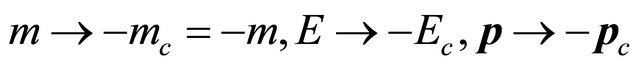
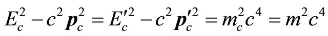
In 1956-1957, the historical discovery of the parity violation [3-6] reveals that both P and C symmetries are violated to maximum in weak interactions. Then in 1964- 1970, both CP and T are experimentally verified to be violated in some cases (though to a tiny degree) [7,8] whereas the product symmetry CPT holds intact to this day [9]. The CPT invariance in quantum field theory (QFT) was first proved by Lüders and Pauli in 1954- 1957 [10-12] via the introduction of the “strong reflection” for proving the CPT theorem. In 1965, Lee and Wu proposed that the definition of particle  versus its antiparticle
  should be [13]
 (1.1)
(1.1)
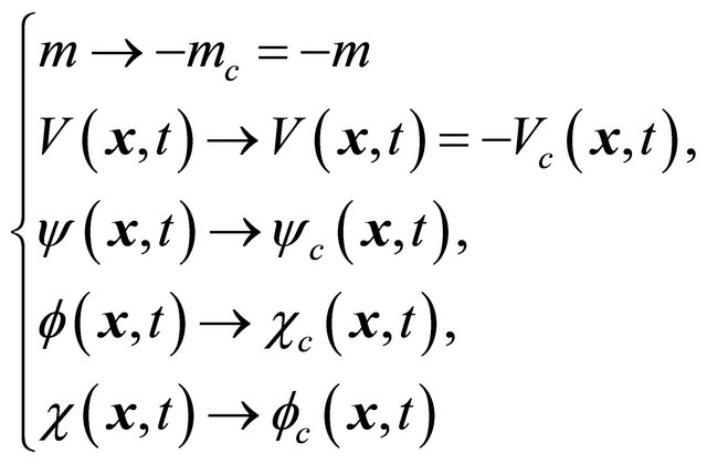
Regrettably, the counterpart of “strong reflection” at the level of RQM went nearly unnoticed in the past decades. In this paper, we are going to study the RQM thoroughly. Not only a discrete symmetry  is found in RQM as the counterpart of “strong reflection” in QFT, it is also evolved into the invariance of space-time inversion
  or mass inversion
  , showing that a WF in RQM is always composed of two parts in confrontation inside a particle and then RQM becomes a self-consistent theory. Furthermore, this symmetry can serve as a “theoretical tool” in searching for new applications in today’s physics.
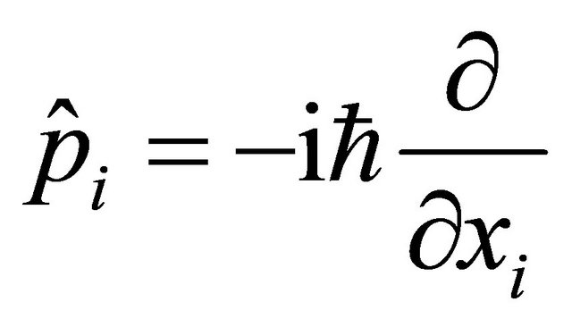
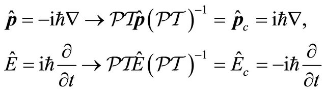
The organization of this paper is as follows: In section II, the EPR paradox [14] is discussed together with the  correlation experimental data [1], yielding a strong hint that the energy-momentum operators for antiparticle’s WF should be
 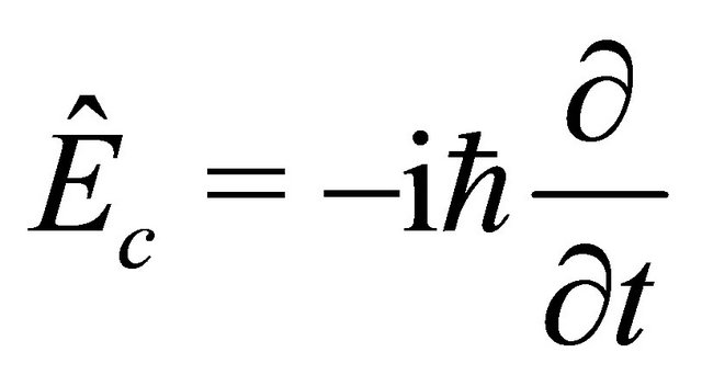 and
and 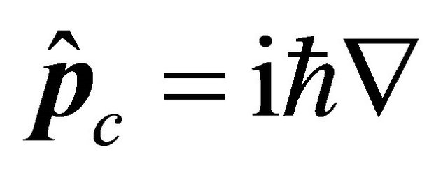 respectively. Section III is focused on a discrete symmetry
 , here
  means the (newly defined) combined space-time inversion (with
 ), while
  the transformation of WFs between particle and antiparticle, whose definition is just residing in the symmetry. Then after combining with FV dissociation of KG equation [2] in which the WF
  is composed of two fields:
 , the above symmetry can be realized in terms of
  and
and  rigorously via the invariance of their coupling equation either under the spacetime inversion or a mass inversion
  In this way, the probability density is ensured to be positive definite for WFs of either particle or antiparticle. Section IV ascribes various phenomena in the theory of special relativity (SR) to the effects of enhancement of the hidden
  field in a moving particle. In Section V, Dirac equation is discussed accordingly with the importance of helicity being stressed. Section VI contains a brief discussion on the QFT. Sections VII, VIII and IX are devoting to seek for possible applications of the above symmetry in today’s physical problems: Why a parity violation phenomenon was overlooked since 1956-1957? Why we believe neutrinos are likely the tachyons? And the prediction of antigravity between matter and antimatter. The last Section X contains a summary. In the Appendix, the Klein paradox is solved for both KG equation and Dirac equation without resorting to the “hole theory”.
2. What the  Correlation Experimental Data Are Telling?
To our knowledge, beginning from Bohm and Bell [15,16], physicists gradually turned their research of EPR paradox [14] onto the entangled state composed of electrons, especially photons with spin and achieved fruitful results. However, as pointed out by Guan (1935-2007), EPR’s paper [14] is focused on two spinless particles and Guan found that there is a commutation relation hiding in such a system as follows [17]:
Consider two particles in one dimensional space with positions  and momentum operators
 . Then a commutation relation arises as
 (2.1)
(2.1)
According to QM’s principle, there may be a kind of common eigenstate having eigenvalues of these two commutative (i.e., compatible)observables like:
 (2.2)
(2.2)
with D being their distance. The existence of such kind of eigenstate described by Equation (2.2) puzzled Guan, he asked: “How can such kind of quantum state be realized?” A discussion between Guan and one of present authors (Ni) in 1998 led to a paper [18].
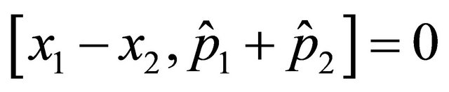
Here we are going to discuss further, showing that the correlation experiment on a  system (which just realized an entangled state composed of two spinless particles) in 1998 by CPLEAR collaboration [1] actually revealed some important features of QM and then answered the puzzle raised by EPR in a surprising way. First, besides Equation (1), let us consider another three commutation relations simultaneously:
 (2.3)
(2.3)
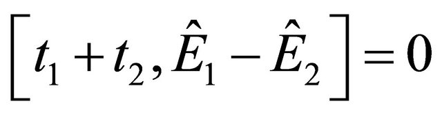
 (2.4)
(2.4)
 (2.5)
(2.5)
( with
with  being the time during which the i-th particle is detected). In accordance with Ref. [1], we also focus on back-to-back events. The evolution of
 ’s wavefunction (WF) will be considered in three inertial frames: The center-of-mass system S is at rest in laboratory with its origin x = 0 located at the apparatus’ center, where the antiprotons’ beam is stopped inside a hydrogen gas target to create
  pairs by
  annihilation. The
  pairs are detected by a cylindrical tracking detector located inside a solenoid providing a magnetic field parallel to the antiprotons’ beam. For back-to-back events, the space-time coordinates in Equations (1)-(5) refer to particles moving to the right
  and left
  respectively. Second, we take an inertial system
  with its origin located at particle 1 (i.e.,
 ).
).  is moving in a uniform velocity
  with respect to
 . (For Kaon’s momentum of
 ). Another
  system is chosen with its origin located at particle
 .
. is moving in a velocity
  with respect to
 . Thus we have Lorentz transformation among the space-time coordinates being
 (2.6)
(2.6)
Here  and
and  correspond to the proper time
  and
and  in Ref.[1] respectively. The common time origin
  is adopted.
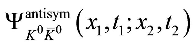
A  pair, created in a
  antisymmetric state, can be described by a two-body WF depending on time as ([1], see also [19,20])
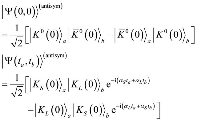 (2.7)
(2.7)
with
 (2.8)
(2.8)
where the CP violation has been neglected and
 ,
,  and
and  being the
  masses and decay widths, respectively. From Equation (7), the intensities of events with like-strangeness (
 or
or ) and unlike-strangeness (
 or
or ) can be evaluated as
 (2.9)
(2.9)
 (2.10)
where  and
and
 or
or .
.
Similarly, for  created in a
  or
or  symmetric state as:
 (2.11)
the predicted intensities read

(2.12)
The experiment [1] reveals that the  pairs are mainly created in the antisymmetric state shown by Equations (2.9) and (2.10) while the contribution in a symmetric state shown by Equations (2.11) and (2.12) accounts for 7.4%.
What we learn from Ref. [1] in combination with Equations (2.1)-(2.5) are as follows:
(a) Because only back-to-back events are involved in the  system, we denote three commutative operators as: the “distance” operator
 and
and , Equations (2.1) and (2.3) read
 (2.13)
So they may have a kind of common eigenstate during the measurement composed of  and projected from the symmetric state shown by Equation (11). It is assigned by a continuous eigenvalue
  (with continuous index
 ) of operator
  acting on the WF,
  , as1
, as1
 (2.14a)
 (2.15)
 (2.16)
where the lowest eigenvalue of  is
is
 , and that of
  is
is
 respectively. These eigenstates of like-strangeness events predicted by Equation (11) are really observed in the experiment [1] (these eigenstates of
  were overlooked in the Ref. [18]).
(b) The more interesting case occurs for  pair created in the antisymmetric state with intensity given by Equation (10) being a function of
  (not
(not  as shown by Equation (12) for symmetric states)
which is proportional to  in the S system. In the EPR limit
 ,
,  events dominate whereas likestrangeness events are strongly suppressed as shown by Equation (9) (see Figure 1 in [1]). So the experimental facts remind us of the possibility that
  events may be related to common lowest (zero) eigenvalues of some commutative operators (just like what happened in Equations (15) and (16) for operators
  and
and  (which are applied to symmetric states (due to
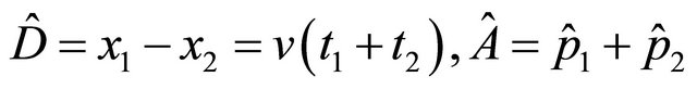
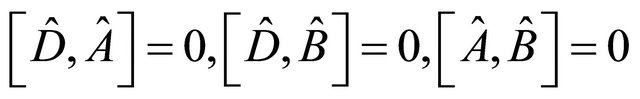
 ) but are not suitable for antisymmetric states), there are another three operators shown by Equations (4) and (5) being: the operator of “flight-path difference”
  and
and
 with commutation relations as:
 (2.17)
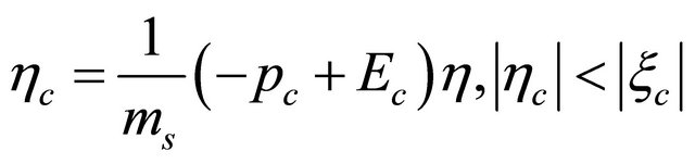
which are just suitable for antisymmetric states. For  back-to-back events, assume that one of two particles, say 2, is an antiparticle with its momentum and energy operators being
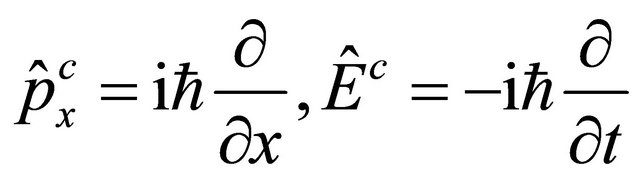 (2.18)
(the superscript  means “antiparticle”) versus that for particle being
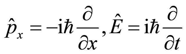 (2.19)
For instance, a freely moving particle’s WF reads2:
 (2.20)
whereas
 (2.21)
for its antiparticle with  and
and  being momentum and energy of the antiparticle in accordance with Equation (2.18). If using Equations (2.18)-(2.21), we find
 (2.22)
with continuous index  referring to continuous eigenvalues
 . Here, the WF in space-time of this system during measurement reads approximately:
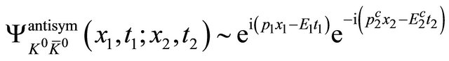 (2.23)
with antiparticle 2 moving opposite to particle 1 and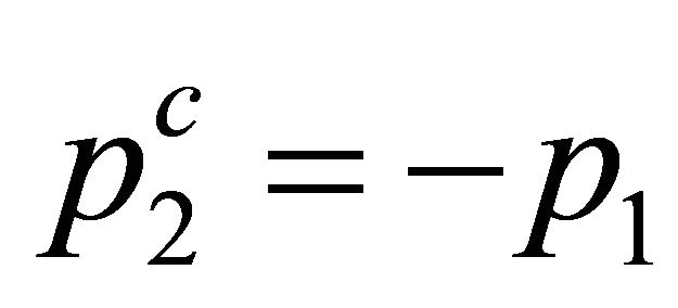 .
.
Now we use  on
on  system, yielding
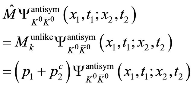 (24)
(24)
Similarly, we have 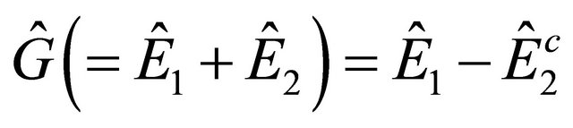 and find
 (25)
(25)
Hence we see that once Equations (2.18) and (2.21)
are accepted, the WFs  show up in experiments as the only WFs with strongest intensity at the EPR limit
 corresponding to their three eigenvalues being all zero:
  and they won’t change even when accelerator’s energies are going up.
If using Equation (2.18), the eigenvalues of  and
and
 for the WF
  are
are
 and
and  respectively, while that of
  and
and  for the WF
 are
are  and
and
 , respectively, those eigenvalues are much higher than zero and going up with the accelerator’s energy.
Something is very interesting here: If we deny Equation (2.18) but insist on unified operators  and
and  for both particle and antiparticle, there would be no difference in eigenvalues between like-strangeness events and unlike-strangeness ones. For example, the
  and
and  would be
  and
and  too (instead of “0” as in Equations (2.24) and (2.25)). This would mean that three commutative operators
  and
and  are not enough to distinguish the WF
  from the WF
  even they behave so differently as shown by Equations (9) and (10)), especially at the EPR limit
 .
.
Equation (2.18) together with the identification of WF
 by three zero eigenvalues implies that the difference of a particle from its antiparticle is not something hiding in the “intrinsic space” like opposite charge (for electron and positron) or opposite strangeness (for
  and
and ) but can be displayed in their WFs evolving in space-time at the level of QM.
In summary, instead of one set of WF with its operators (Equations (2.19) and (2.20)), two sets of WFs with operators separately (shown as Equations (2.18)- (2.21)) are strongly supported by the original EPR paradox and its “solution” provided by the  experiment.
To our knowledge, Equation (2.18) can be found at a page note of a paper by Konopinski and Mahmaud in 1953 [21], also appears in Refs. [18,22-28].
3. How to Make Klein-Gordon Equation a Self-Consistent Theory in RQM? A Discrete Symmetry
3.1. The Negative Energy Solution and the WF of Antiparticle
Let us begin with the energy conservation law for a particle in classical mechanics:
 (3.1)
(3.1)
Consider the rule promoting observables into operators:
 (3.2)
(3.2)
and let Equation (3.1) act on a wavefunction (WF) , the Schrödinger equation
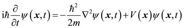 (3.3)
(3.3)
follows immediately. In mid 1920’s, considering the kinematical relation for a particle in the theory of special relativity (SR):
 (3.4)
(3.4)
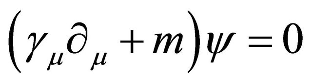
and using Equation (3.2) again, the Klein-Gordon (KG) equation was established as:
 (3.5)
(3.5)
For a free KG particle, its plane-wave solution reads:
 (3.6)
(3.6)
However, two difficulties arose:
(a) The energy E in Equation (6) has two eigenvalues:
 (3.7)
(3.7)
In general,  , the WFs of KG particle’s energy eigenstates can always be divided into two parts:
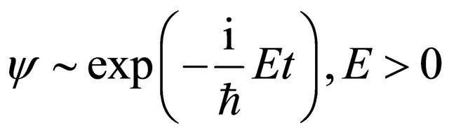 (3.8)
(3.8)
 (3.9)
(3.9)
where only the original operators Equation (3.2) are used. But what the “negative energy” means?
(b) The continuity equation is derived from Equation (5) as
 (3.10)
where
 (3.11)
and
 (3.12)
are the “probability density” and “probability current density” respectively. While the latter is the same as that derived from Equation (3.3), Equation (3.11) seems not positive definite and dramatically different from  in Equation (3.3). Why?
In hindsight, for a linear equation in RQM, either KG or Dirac equation, the emergence of WFs with both positive and negative energy  is inevitable and natural. From mathematical point of view, the set of WFs cannot be complete if without taking the negative energy solutions into account. And physicists believe that these negative-energy solutions might be relevant to antiparticles. However, we physicists admit that both a rest particle’s energy
  and a rest antiparticle’s energy
  are positive, as verified by numerous experiments like that of pair-creation process
  . The above contradiction constructs socalled “negative-energy paradox” in RQM. For Dirac particle, majority (not all) of physicists accept the “hole theory” to explain the “paradox”. But for KG particle, no such kind of “hole theory” can be acceptable. It was this “negative-energy paradox” as well as the four “commutation relations”, Equations (2.1)-(2.5), hidden in the two-particle system discussed by EPR [14] gradually prompted us to realize that the root cause of difficulty in RQM lies in an a priori notion—only one kind of WF with one set of operators (like Equation (3.2)) can be acceptable in QM, either for NRQM or RQM.
Once getting rid of the constraint in the above notion and introducing two sets of WFs and operators for particle and antiparticle respectively, we can identify the negative energy solution, Equation (3.9), with the antiparticle’s WF directly
 (3.13)
which implies an antiparticle with positive energy  by using Equation (2.18). This claim will be proved rigorously in the next subsection.
One may ask: When you assume the negative energy solution being the WF of antiparticle, how about the difficulty of negative probability density? Below we will see how to solve these two difficulties simultaneously and make KG equation a self-consistent theory at the level of RQM.
3.2. The Proof of a Discrete Symmetry  for KG Particle
Let us introduce an operator of (newly defined) combined space-time inversion  for KG equation. It should change the space-time coordinates as
 (3.14)
then accordingly
 (3.15)
Because the antiparticle has opposite charge  versus
  for particle, so
 (3.16)
When performing  inversion on KG equation, Equation (3.5), from left to right, we meet eventually the WF and define the antiparticle’s WF as
 (3.17)
Thus KG particle’s equation, Equation (3.5), is transformed into 
 (3.18)
or
 (3.19)
which is formally the same as Equation (3.5) though we should use  for
for . Hence the KG equation remains invariant under the
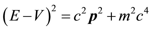
  operation, Equations (3.14)-(3.17). Notice further that Equation (3.18) is just the “quantized” equation of the kinematical relation for an antiparticle in SR
 (3.20)
which is the counterpart of Equation (3.4) for a particle. For example, a KG particle’s scattering WF  is attracted by an spherically symmetric potential
  and so has a positive phase-shift
  (in the, say,
  state). Then physically, its antiparticle’s WF
 is repelled by the potential
  and has a negative phaseshift
 .
.
Note that, however, corresponding to , there is another negative energy particle’s WF
 satisfying Equation (3.5)
 (3.21)
whose space-time behavior is precisely the same as the antiparticle’s WF  with
with 
as shown by Equation (3.18) since
 . Thus, for avoiding confusion, we have
 (3.22)
and
 (3.23)
achieving the proof of the discrete symmetry  for KG particle shown by Equation (3.17). In summary, the “negative-energy paradox” for KG equation is solved in a physical way with following advantages:
a) By using two sets of WFs and momentum-energy operators for particle and antiparticle respectively, both particle’s WF  and antiparticle’s WF
  have positive energies
  and
and  respectively.
b) While satisfying the same KG equation with same potential  formally,
  and
and  are actually subject to opposite “force” for particle and antiparticle respectively.
c) The space-time behavior of  can be identified with that of a negative energy particle’s WF
 , in a one-to-one correspondence.
Thus from mathematical point of view, all solutions of KG equation form a complete set including both positive and negative energy values of one operator 
exactly.
By contrast, usually, aiming at finding an anti-particle’s WF, one performs the CPT transformation on a particle’s WF , yielding [29-32]
 (3.24)
whose character can also be summed up as follows:
a’) By using one set of WF and relevant operators for both particle and antiparticle, at the LHS of Equation (3.24),  , and
, and  at RHS must have opposite energies inevitably.
b’) By design in the C transformation,  and
and  in Equation (3.24) satisfy different equations with
  and
and  respectively. But with opposite energies, they are actually subject to the same (either attractive or repulsive) “force”. So one cannot distinguish particle from antiparticle through what their WFs “feel” after the CPT transformation.
c’) From mathematical point of view, we should keep all negative-energy solutions for one equation. However, even facing WFs in doubled numbers, we still don’t know how to choose half of them for describing particle and its antiparticle separately in physics.
But we haven’t solve the difficulty of negative probability density in KG equation yet, awaiting for another enlightenment which was already there since 1958.
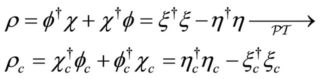
3.3. Feshbach and Villars (FV) Dissociation of KG WF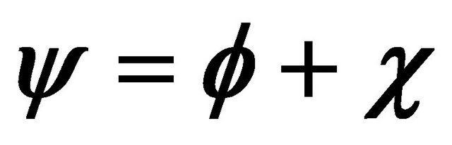 , a Reformulated Symmetry between
  and
and  under the Space-Time (or Mass) Inversion
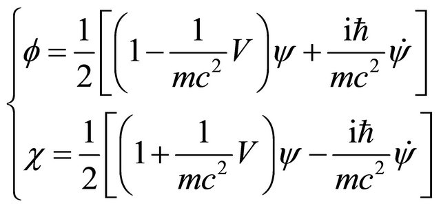
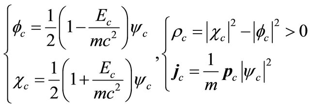
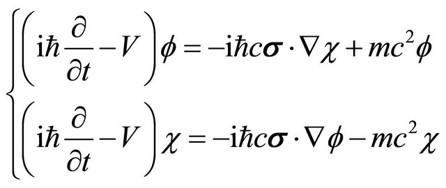
In 1958, dividing the WF into , Feshbach and Villars [2] recast Equation (5) into two coupled Schrödinger-like equations as3:
 (3.25)
where
 (3.26)
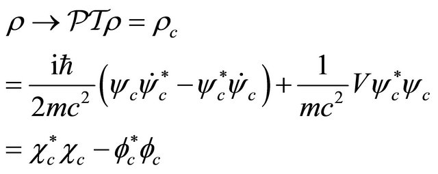
 . Interestingly, the “probability density”, Equation (3.11) can be recast into a difference between two positive-definite densities [18,20]:
 (3.27)
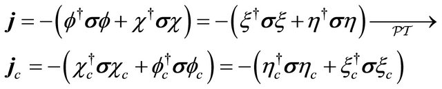
while the probability current density contains interference terms between  and
and :
:
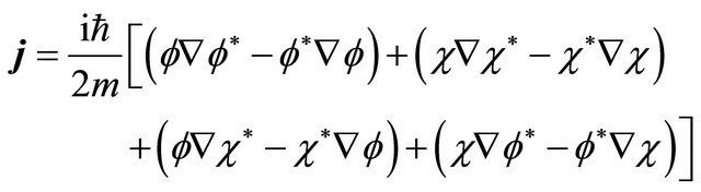 (3.28)
The expression of  as shown by Equation (3.27) strongly hints that the
  symmetry proved in the last subsection may be combined with the FV dissociation of KG equation such that the positive-definite property of
  can be ensured for both particle and antiparticle.
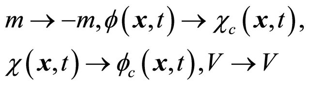
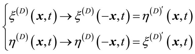
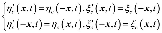
Indeed, after inspecting Equation (3.25) carefully, we do find a hidden symmetry in the sense that it is invariant (in its form) under the following reformulated space-time inversion , i.e.,
  transformation:
 (3.29)
Performing transformation Equation (3.29) on Equation (3.26), we find  satisfying the same equation of
  and
and  satisfying that of
 . They read
 (3.30)
Remember, for , we should use operator Equation (3.15). Accordingly, the probability density for
  is defined as
 (3.31)
Similarly, we have 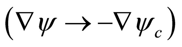
 (3.32)
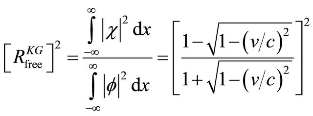
For simplicity, consider a free KG particle  with WF Equation (3.6). Then
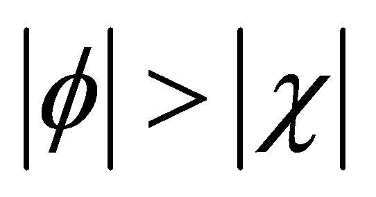
 (3.33)
But for a free  KG antiparticle with WF Equation (2.21), it has
 (3.34)
Equations (3.33) and (3.34) satisfy all physical conditions we need. If , as long as
  for particle or
  for antiparticle, the situation remains the same. However, once
  or
or , some complications would occur. For further discussion, please see the Appendix.
Therefore, we see that the reformulated space-time inversion, Equation (3.29), reflects the underlying symmetry between a particle’s WF  and its antiparticle’s WF
 . As both
  and
and  in
in  or
or  and
and  in
in  are positive definite, all difficulties in KG equation disappear and the latter becomes a self-consistent theory.
Moreover, instead of Equation (3.29), a “mass inversion ” can realize the same symmetry, the invariance under a
  transformation, via the following operation on Equation (3.25):
 (3.35)
Notice that, when , we have
  and
and
 , i.e.
 ,
,  , in contrast to Equation (3.15) [1].4
The reason why  in the space-time inversion Equation (3.29) whereas
  in the mass inversion Equation (3.35) can be seen from the classical equation: The Lorentz force F on a particle exerted by an external potential
  reads:
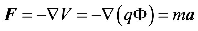 . As the acceleration
  of particle will change to
  for its antiparticle, there are two alternative explanations: either due to the inversion of charge
  (i.e.,
  but keeping
  unchanged) or due to the inversion of mass
  (but keeping
  unchanged).
4. Reinterpretation of WF and the Relativistic Effects
The success of FV’s dissociation of KG equation should be ascribed to their deep insight that a unified WF  is composed of two fields
  and
and  in confrontation. Note that Equation (3.25) reduces into two equations separately for a static KG particle
 :
:
 (4.1)
(4.1)
with two separated solutions being:
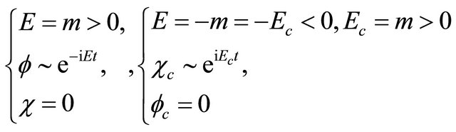 (4.2)
(4.2)
Once the particle (antiparticle) is moving with a velocity,  ,
,  and
and  (
( and
and ) couple together and the WF
 for a free particle (antiparticle) read (in one-dimensional space)
 (4.3a)
 (4.3b)
 respectively. In Equation (4.3a),
  dominates
 . By contrast, in Equation (4.3b) it is
  who dominates
  (The status remains the same for
  cases as discussed in the last section).
Despite  and
and  (
( and
and ) having the “intrinsic tendency” to evolve as
 , however, in a WF of particle (antiparticle),
  must follow
  to evolve like that shown by Equation (4.3a) (Equation
(4.3b)), as . So it seems suitable to name
  the “hidden particle field” inside a particle while
  the “hidden antiparticle field” (rather than the “negative-energy component”) inside the same particle.
Let us try to reinterpret the phenomena displayed in the kinematics of special relativity (SR) via the enhancement of  field in a particle [22-25]:
(a) Lorentz transformation Consider a particle’s WF shown by Equation (4.3a) in an inertial frame S (laboratory). Then take another  frame resting on the particle, so
  and
and  . The WF in
  frame reads:
 (4.4)
(4.4)
Here the space-time coordinates  are introduced and defined in the
  frame via the phase of WF as follows: Based on the assertion that “phase remains invariant under the coordinate transformation” which was named the “law of phase harmony” by de Broglie and was regarded by himself as the fundamental achievement all his life [34], comparing the phase in Equation (4.4) with that in Equation (4.3a) and using
 , one finds
 (4.5)
(4.5)
Then, all formulas in the Lorentz transformation can be obtained. In some sense, what used here is a particle’s wave-packet which serves as a microscopic “ruler”, also a “clock” simultaneously.
(b) There is a speed limit c for a massive particle.
For a free KG particle, using Equation (3.33), we may define an “impurity ratio”  for the amplitude of hidden
  field to that of
  field and calculate it being
 (4.6)
(4.6)
When , with the increase of v,
  increases monotonously. The particle becomes more and more “impure” until
  as a limit of particle being still a particle. As shown by Equation (4.6), the reason why its velocity has a limiting value c (the speed of light) is because
  and
and  have opposite evolution tendencies in space-time as shown by Equations (4.1)- (4.3) essentially,
  strives to hold
  back from going forward until a balance nearly reached when
  and
and .
.
(c) The “length contraction” (FitzGerald-Lorentz contraction) and “time dilation”
As usual, we will show “length contraction” via a wave-packet of KG particle moving at a high-speed  but further ascribe it to the enhancement of
  field hidden inside the particle.
First, consider a wave-packet of KG particle at rest [25, 35]
 (4.7)
(4.7)
Assuming , we have approximately that
 (4.8)
(4.8)
If , the diffusion of wave-packet at low speed
  can be ignored. Then we perform a “boost transformation”

to push the wave-packet to high velocity , yielding
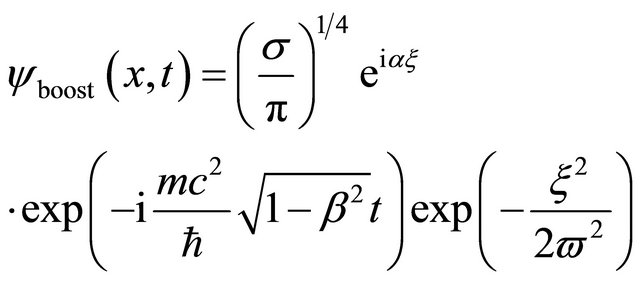 (4.9)
(4.9)
where 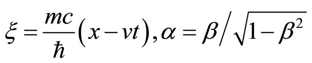 and
and
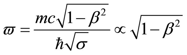 (4.10)
Here  is the width of wave-packet measured from its center
 . Equations (4.7)-(4.10) show the “length contraction”.
Second, we calculate from Equations (4.9) and (3.33)
the values of  and the probability density
 respectively.5 Their peak values all increase with the increase of v (boost effect). However, the “intensity” of
  or
or  increases even faster than that of
  while keeping the constraint
  in the boosting process.
We also calculate the square of “impurity ratio”  for this moving wave-packet:
 (4.11)
which is the counterpart of Equation (4.6) for a plane WF of KG particle.
With these calculations, we might intuitively understand the length contraction as an effect of coupling (i.e. entanglement) between  and
and  fields due to their opposite evolution tendencies in space as discussed in previous point (b).
Let’s turn to the “time dilation” shown by the variation of the mean life
 (4.12)
of a particle, say, a pion ( or
or ) with its velocity
 .
.
To understand it, let’s return back to Equations (4.1)- (4.3) at  and view the WF
  on its complex plane with
  and
and  (
( and
and ) as abscissa and ordinate. We may see that the time reading of the “inner clock” for a particle (or an antiparticle) is “clockwise” (or “counter clockwise”). Thus with the increase of particle velocity, though the time reading remains clockwise (due to the dominance of
  field), it runs slower and slower because of the enhancement of hidden
  field.
(d) WF’s group velocity  versus phase velocity
 .
.
In RQM, a particle’s velocity  should be identified with its group velocity
 . Actually, we have
 (4.13)
However, the fact that there is an upper bound for particle’s velocity doesn’t mean that no speed can exceed that of light, . Indeed, there is another velocity
 , the phase velocity in the WF
 (4.14)
And the relation  implies that
 (4.15)
In our opinion, the role of  here is crucial to maintain the quantum coherence of WF in the space-time globally, we will further discuss this problem elsewhere. In 1923, de Broglie discovered Equation (4.15) in his relativistic theory. However, in the Schrödinger equation of NRQM, the phase velocity remains undefined. See Ref [34].
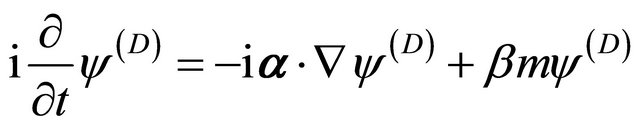
5. Dirac Equation as Coupled Equations of Two-Component Spinors
Let us turn to the Dirac equation describing an electron
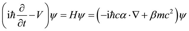 (5.1)
(5.1)
with  and
and  being
being  matrices, the WF
  is a four-component spinor
 (5.2)
(5.2)
Usually, the two-component spinors  and
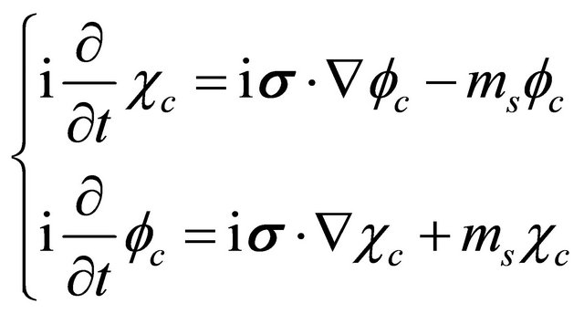
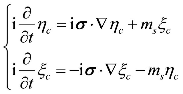
and  are called “positive” and “negative” energy components. In our point of view, they are the hiding “particle” and “antiparticle” fields in a particle (electron) respectively ([25], see below). Substitution of Equation (2) into Equation (1) leads to
 (5.3)
(5.3)
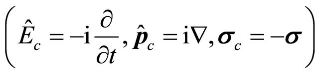
( are Pauli matrices). Equation (3) is invariant under the combined space-time inversion with
 (5.4)
(5.4)
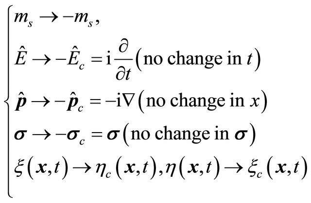
showing that in its form of two-component spinors, Dirac equation is in conformity with the underlying symmetry Equation (3.29). Note that under the space-time inversion, the  remain unchanged (However, see Equations (9)- (11) below). Alternatively, Equation (3) also remains invariant under a mass inversion as
 (5.5)
(5.5)
In either case of Equation (5.4) or (5.5), we have6
 (5.6)
(5.6)
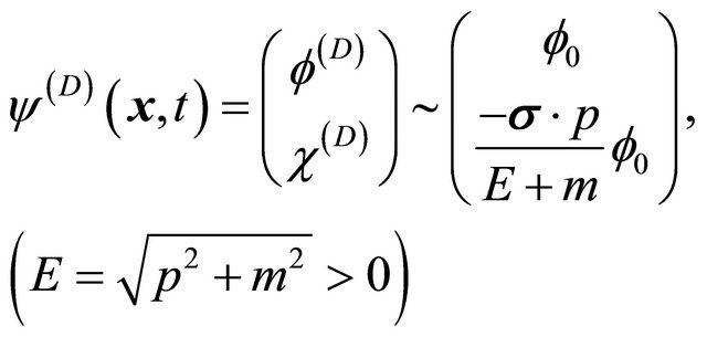
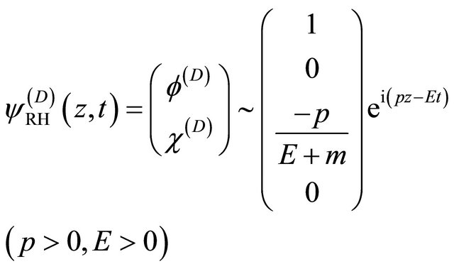
For concreteness, we consider a free electron moving along the z axis with momentum  and having a helicity
 , its WF reads:
 (5.7)
(5.7)
with . Under a space-time inversion
 or mass inversion
 , it is transformed into a WF for positron (moving along
  axis)
axis)
 (5.8)
(5.8)
with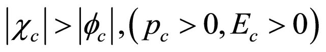 . However, the positron’s helicity becomes
 . This is because the total angular momentum operator for an electron reads
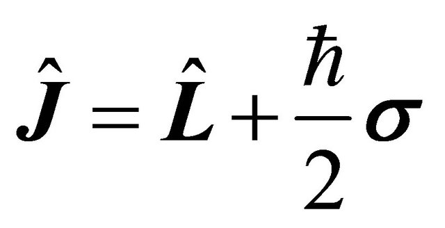 (5.9)
(5.9)
Under a space-time inversion, the orbital angular momentum operator is transformed as
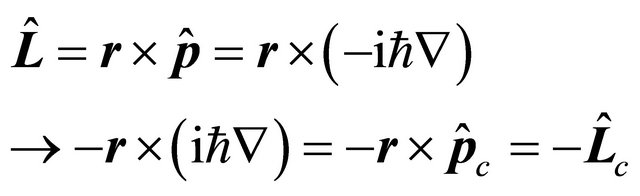 (5.10)
To get  with
with , we should have
 (5.11)
Hence the values of matrix element for positron’s spin operator  is just the negative to that for
  in the same matrix representation.
Notice that Equation (7) describes an electron with positive helicity, i.e.,  7. Under a space-time inversion, it is transformed into
 in Equation (8), i.e.,
 , meaning that Equation (8) describes a positron with negative helicity.
In its form of four-component spinor, Dirac equation, Equation (5.1) with , is usually written in a covariant form as (Pauli metric is used:
 , see Ref. [25]):
 (5.12)
Under a space-time (or mass) inversion, it turns into an equation for antiparticle:
 (5.13)
with an example of  shown in Equation (8). Let us perform a representation transformation:
 (5.14)
and arrive at
 (5.15)
due to . Since
  and
and  are essentially the same in physics, (this is obviously seen from its resolved form, Equation (5.3)), it is merely a trivial thing to change the position of
  in the 4-component spinor (lower in Equation (5.14) and upper in Equation (5.8)).
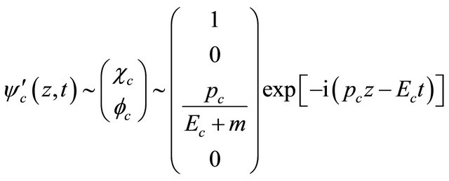
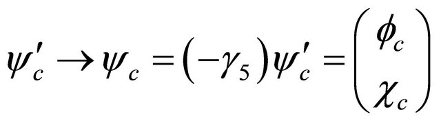
What important is  for characterizing an antiparticle versus
  for a particle. Therefore, if a particle with energy E runs into a potential barrier
 , its kinetic energy
 becomes negative, and its WF’s third component in Equation (5.7) suddenly turns into
 , whose absolute magnitude is larger than that of the first component. This means that it is an antiparticle’s WF satisfying Equation (5.15) (with
  and
and ) and will be crucial for the explanation of Klein paradox in Dirac equation (For detail, please see Appendix). However, we need to discuss the “probability density”
  and “probability current density”
  for a Dirac particle versus
  and
and  for its antiparticle. Different from that in KG equation, now we have
 (5.16)
which is positive definite for either particle or antiparticle. On the other hand, we have
 (5.17)
(we prefer to keep  rather than
  for antiparticle). For Equations (5.7), (5.8) and (5.14), we find
 (5.18)
which means that the probability current is always along the momentum’s direction for either a particle or antiparticle.
Above discussions at RQM level may be summarized as follows: The first symptom for the appearance of an antiparticle is: If we perform an energy operator
 on a WF and find a negative energy
 or a negative kinetic energy
 , we’d better doubt the WF being a description of antiparticle and use the operators for antiparticle, Equation (2.18). Then for further confirmation, two more criterions for
  and
and  are needed (see Appendix).
6. The Strong Reflection Invariance in CPT Theorem and QFT
In QFT, the starting point is the field operator which is constructed for free complex boson field as [36]
 (6.1)
(6.1)
Similarly, the field operator for free Dirac field reads:

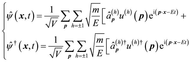 (6.2)
(6.2)
In Equation (6.1), the annihilation operator  for particle and the creation operator
  for antiparticle in Fock space are introduced. In Equation (6.2), instead of index
  (
( , the spin’s projection along the fixed
  axis in space), the helicity
  is used. See Ref. [37].
Let us return back to the CPT theorem proved by Lüders and Pauli in 1954-1957 [10-12]. The proof of CPT theorem contains a crucial step being the construction of so-called “strong reflection”, consisting in a reflection of space and time about some arbitrarily chosen origin, i.e. .
.
Pauli proposed and explained the strong reflection in Ref. [12] as follows: When the space-time coordinates change their sign, every particle transforms into its antiparticle simultaneously. The physical sense of the strong reflection is the substitution of every emission (absorption) operator of a particle by the corresponding absorption (emission) operator of its antiparticle. And there is no need to reverse the sign of the electric charge when the sign of space-time coordinates is reversed.
What Pauli claimed, in our understanding, means that under the strong reflection for boson field, one has
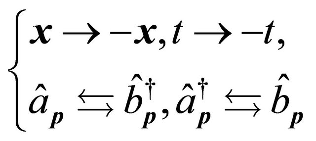 (6.3)
(6.3)
The mutual transformation, Equation (6.3), in Fock space ensures the field operators, Equation (6.1), invariant under the strong reflection in the sense of (see also [25,26]):
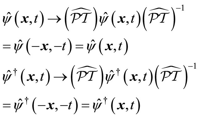 (6.4)
(6.4)
Here let us introduce the notation  to represent the strong reflection so that the presentation could be easier and clearer as shown above. Similarly, for Dirac field, under the strong reflection one has
 (6.5)
(6.5)
Here it is important to notice that the helicity,  , will be reversed before and after the strong reflection for a particle and its antiparticle respectively as discussed in Section V. Because Equation (6.2) is written in 4 component spinor covariant form, the invariance of Dirac field operator under the strong reflection should be expressed rigorously as
 (6.6)
(6.6)
 (6.7)
(6.7)
which are useful in proving the “spin-statistics connection” by strong reflection invariance.
QFT is a successful theory just because it is established on sound basis with the field operator being one of its cornerstones. Historically, through various trials and checks, Equations (6.1)-(6.2) were eventually found (see Section 3.5 of Ref. [36]). Why they are correct and why one would fail otherwise? In our understanding, it is just because they are invariant under the strong reflection as shown by Equations (6.4) and (6.6).
However, as emphasized by Pauli [12] and further stressed by Lüders [11], at least two more rules should be added in doing calculations:
(a) The order of an operator product in Fock space has to be reversed under the strong reflection, e.g.,
 . So is the order of a process occurred in a many-particle system.
(b) Another rule is: One should always take the normal ordering when dealing with quadratic forms like  etc.
etc.
Then Pauli and Lüders were able to prove that the Hamiltonian density  for a broad kind of model in relativistic QFT is invariant under an operation of “strong reflection”, i.e.,
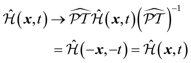 (6.8)
(6.8)
The Hamiltonian density is also invariant under a Hermitian conjugation (H.C.) as:
 (6.9)
(6.9)
Furthermore, they proved the CPT theorem via the identification of the product of T, C, and P in QFT with the combined operation of the strong reflection and a Hermitian conjugation.
The validity of CPT invariance, i.e. Equations (6.8) and (6.9) has been verified experimentally since the discovery of parity violation ([3-8] etc.) and the establishment (and development) of standard model ([38] etc.) in particle physics till this day. See the excellent book, Ref. [19] and the Review of Particle Physics, Ref. [9].
After restudying the historical contribution of PauliLüders strong reflection invariance, we feel good in understanding that what we claim in RQM (Sections III-V) is essentially the same as or very close to their idea.
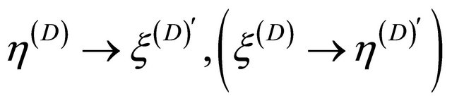
In fact, this paper is the direct continuation of our first one in 1974 [22], which was inspired jointly by the discoveries of violations in P, C, CP, T symmetries individually (but CPT invariance holds), also by Lee-Wu’s proposal in 1965 that the relationship between a particle  and its antiparticle
  should be [13]:
 (6.10)
and especially by Pauli’s invention of the strong reflection in 1955 [12].
Below, we would like to show that WFs for a particle and its antiparticle given in Equations (5.7) and (5.8) are precisely that derived from QFT as expected.
Using Equation (6.2) for Dirac field, we find the WF of an electron being
 (6.11)
but the hermitian conjugate of a positron’s WF is given by
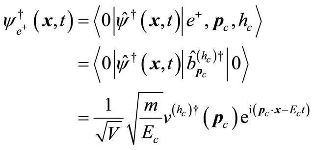 (6.12)
which leads to positron’s WF being
 (6.13)
Similarly, Equations (2.20) and (2.21) can be derived from Equation (6.1) as expected.
7. An Oversight in QFT (Helicity States or Spin States?)—Why a Parity-Violation Phenomenon Was Overlooked Since 1956-1957?
Through analysis in RQM till QFT, we stress the necessity of using helicity  to describe a fermion or antifermion. Here is an interesting example. Since 2002, Shi and Ni [39-43] predicted a parity-violation phenomenon as follows:
An unstable (decaying) fermion (e.g., neutron or muon) has different mean lifetimes for being right-handed (RH) or left-handed (LH) polarized during its flight with the same speed 
 (7.1)
(7.1)
where ,
,  the mean lifetime when it is at rest. Similarly, for its antifermion, their lifetimes will be
 (7.2)
(7.2)
Hence, the lifetime asymmetry can be defined as
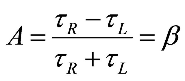 (7.3)
(7.3)
This is not a small effect. For instance, in Fermilab, physicists consider to build a muon collider [44]. The collision of  and
and  beams must happen before the muons decay. It was estimated that if a muon rings along at 1.5 TeV, the time dilation of SR stretches its lifetime to 30 milliseconds—up from 2 microseconds when it’s still. That’s time enough for 500 circuits in the final ring. However, as discussed in Ref. [43], if the prediction of life asymmetry Equation (7.1) is correct, the lifetime of RH
  will be stretched to 146 days while that of LH
  only 15 milliseconds. The lifetime asymmetry of
  will be just the opposite as shown by Equation (7.2). Therefore, it seems necessary to take Equations (7.1)- (7.2) into account in the design of a muon collider.
The problem is: How can such a parity-violation phenomenon be overlooked since 1956-1957? One theoretical reason is: in the past, for describing a fermion in flight , instead of helicity states, the “spin-states” assigned by
  (spin’s projection along the fixed
  axis in space) were often incorrectly used (see [40-42]). So previous calculations on the lifetime always led to a prediction that
 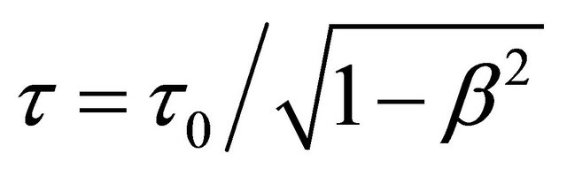 without parity-violation in contrast to Equations (7.1)-(7.3).8
The interesting thing is: While Equations (7.1) and (7.2) display the violation of P or C symmetry to its maximum, their “cross-symmetry”,  and
and  , reflects the symmetry of
  shown by Equation (6.5) exactly.
8. Dirac Particles Conserve the Parity Whereas Neutrinos Are Likely the Tachyons
8.1. Why Dirac Equation Respects the Parity Symmetry?
In the standard representation of Dirac equation for free particle 
 (8.1)
(8.1)
Let us choose
 , then
 (8.2)
(8.2)
As discussed in section V, Equations (8.1) and (8.2) are invariant under the space-time inversion:
 (8.3)
(8.3)
with subscript “c” meaning the antiparticle.
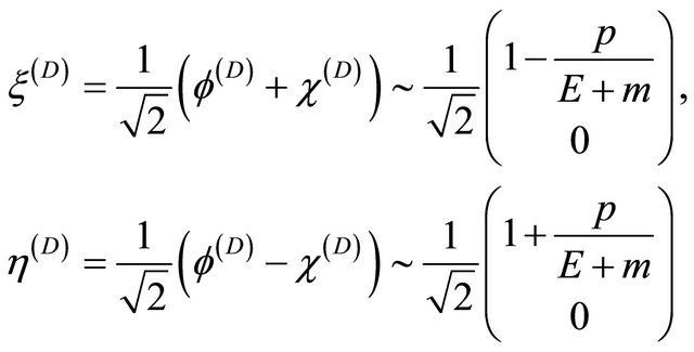
After transforming  into the “Weyl representation” (chiral representation) as
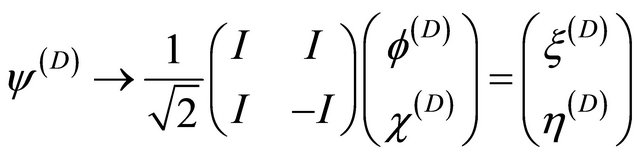 (8.4)
(8.4)
we have
 (8.5)
(8.5)
If , Equation (8.5) reduces into two Weyl equations describing two kinds of permanently LH and RH polarized massless fermions respectively. So we may name
  and
and  (which are usually called as chirality states or chiral fields in 4-component covariant form) as the “hidden LH and RH spinning fields” inside a Dirac particle, which can be either LH or RH polarized (with helicity
  or 1) explicitly. See below.
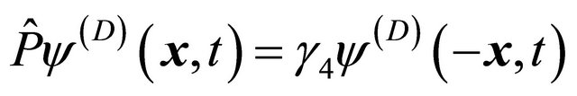
A new symmetry is hidden in Equation (8.5), which remains invariant under the pure space inversion  transformation, i.e., the parity operation as
 (8.6)
(8.6)
Here we add “ ” in the superscript of RHS to stress that the WF after the space inversion may be different from that at the LHS (before the space inversion). We knew that the WF in Dirac representation after a space inversion reads
 (8.7)
(8.7)
Using Equation (8.6), the RHS of Equation (8.7) turns out to be
 (8.8)
(8.8)
Hence, we understand the reason why a Dirac particle respects the parity symmetry as shown by Equation (8.7) is because it enjoys the symmetry Equation (8.6) hiding in the 2-component spinor form (in Weyl representation).
For concreteness, let’s write down the solution of Equation (8.1)
 (8.9)
(8.9)
Furthermore, we choose a simplest “spin state” with
 and
and :
:
 (8.10)
While Equation (8.10) is an eigenfunction of  with eigenvalue
 , its helicity
  remains unfixed, depending on the value of
  being positive or negative. Only after
  is fixed, can we have a “helicity state” describing a RH particle with
 :
:
 (8.11)
Looking at Equation (8.11) in the Weyl representation, we see that
 (8.12)
 . So Equation (8.11) describes a RH particle just because the
  field dominates the
  field. Now we perform a space inversion on Equation (8.11), according to the rule Equation (8.7), yielding

(8.13)
Hence we see that the reason why  becomes a LH WF, i.e.,
 (8.14)
is just because of the dominance of  field over
 field after the P-operation. Before and after the operation,
  , the dominant (subordinate) field is transformed into dominant (subordinate) field:
 , as shown by Equation (8.6).
In summary, Dirac equation is invariant under a space inversion whereas its concrete solution of WF may be not. The latter may change from that for a RH particle to a LH one or vice versa, but with the same mass m, showing the law of parity conservation exactly.
8.2. Tachyon Equation as a Counterpart of the Dirac Equation
Now a question arises: Can we find an equation which violates the symmetry of pure space inversion?
The answer is “yes”. Let’s introduce a new equation in Weyl representation from Equation (8.5) by erasing the superscript (D), replacing the mass term by  and changing its sign from “+” to “−” in the first equation of Equation (8.5) only [46]
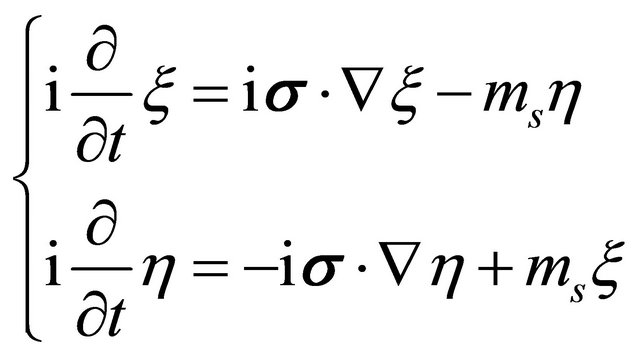 (8.15)
where  (real and positive) refers to the mass of a hypothetical particle. We will see immediately that it is a “superluminal particle” or “tachyon”.
Indeed, substituting a plane-wave solution
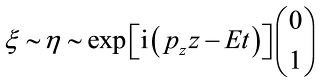 (8.16)
with the particle’s helicity  into Equation (8.15), we find that
 (8.17)
 (8.18)
Since  and
and , from Equation (8.17), the dispersion-relation of wave reads
 (8.19)
As in Section IV, we define the wave’s phase velocity  as
as
 (8.20)
while its group velocity 
 (8.21)
being identical with the particle’s velocity . Equation (8.19) yields a relation between them coinciding with Equation (4.15) exactly:
 (8.22)
However, the relations among  and
and  are dramatically different
 (8.23)
which dictate  such that
  are real and
 .
.
Like Equation (8.4), we define:
 (8.24)
and find from Equation (8.15) that (in Dirac representation)
 (8.25)
 (8.26)
 . Despite the difference between Equation (8.26) and Dirac equation, Equation (8.2), both of them respect the combined space-time inversion
  symmetry like Equation (8.3)
 (8.27)
with
 (8.28)
Similarly, we define the WF in Weyl representation after  inversion as:
 (8.29)
Based on Equations (8.27)-(8.29), we find
 (8.30)
 (8.31)
which can also be obtained via the  operation on Equation (8.15). Equations (8.15) and (8.31) are better to be compared in the following form:
 (8.32)
 (8.33)
 . Interestingly, Equation
(8.33) can also be reached from Equation (8.32) via a “mass inversion” like that in Sections III and V:
 (8.34)
Furthermore, the probability density and probability current density before and after the  inversion can be derived as:
 (8.35)
and
 (8.36)
respectively. It is the sharp contrast between Equation (8.35) and Equation (5.16) for Dirac equation (i.e.,
 ), that makes Equation (8.15)
so unique as shown below.
Let us look at the example of WF for tachyon, Equations (8.16)-(8.18), with  and
and . It is allowed just because
  and so
 . Second choice of Equation (8.16) with
 but
but
 (8.37)
should be fobidden due to its ρ < 0. Another two possible WFs with  have
have  and
and  respectively, only the last one with
 is allowed due to its
 and
and .
.
Let us turn to the solution of Equation (8.31) for antitachyon with  by just performing
  operation on Equation (8.16) yielding:
 (8.38)
Now if , since
 , so helicity
 . Substitution of Equation (8.38) into Equation (8.33) yields:
 (8.39)
which is allowed due to . Second choice of Equation (8.38) with
  but
but
 (8.40)
should be forbidden due to its . In another two possible WFs with
 , only that with
 is allowed due to
 .
.
Hence we see that: The tachyon can only exist in a left-handed (LH) polarized state (with helicity ) whereas antitachyon only in a right-handed (RH) polarized state (with
 ). We tentatively link this strange feature with that found in neutrinos—only
  and
and  exists in nature whereas
  and
and  are strictly forbidden.
Furthermore, at first sight, although Equation (8.15) certainly has no symmetry under the space inversion , it seems to enjoy a pure “timeinversion”
  symmetry like
 (8.41)
 (8.42)
We add “ ” in the superscript of
  to stress that
  (being a time reversed WF), though looks like some antitachyon’s WF, is obviously different from
  gained through the
  inversion, Equation (8.31). Actually, based on Equations (8.29)-(8.31) and (8.41)-(8.42), we have:
 (8.43)
Interestingly, we cannot find from Equation (8.42) the “physical solution” of  with
with  (so
(so ) and
) and  (for
(for ) simultaneously. Only
  makes physical sense, but it is just
  like that discussed in Equation (8.39). Notice that the sign change
  in the phase of WF makes a change in the direction of momentum
 . But a WF is always composed of two fields in confrontation, like
  versus
  here. And the explicit helicity
  is determined by which one of these two hidden fields being in charge. So the change of
  in these four equalities of Equation (8.43) does reverse the status of
  versus
  (or
(or  vs
vs ), rendering helicity reversed explicitly. The subtlety of tachyon equation, unlike Dirac equation, lies in the fact that only
  and
and  exist whereas
  and
and  are strictly forbidden, i.e., the parity symmetry is violated to maximum. Hence, in strict sense, there is also no physically meaningful WF after the operation of pure “time inversion” on Equation (8.15). We will insist on Equation (8.31) rather than Equation (8.42)—there is only one correct way leading from tachyon to antitachyon via the
  inversion essentially.
In 2000, Equation (8.25) was first proposed by Tsao Chang and then collaborated with Ni in Ref. [46] (see also [47-52] and the Appendix 9B in Ref. [25]). At first sight, the difference between Equations (8.25) and (8.1) amounts to substituting the mass term  by
by 
with  being an antihermitian matrix.
Usually, for an equation with nonhermitian Hamiltonian, there is no guarantee for the completeness of its mathematical solutions. In other words, the unitarity of its physical states is at risk. Sometimes, however, a nonhermitian Hamiltonian can be accepted in physics. For example, in the optical model for nuclear physics, an imaginary part of potential,  , is used to describe the absorption of incident particles successfully. The interesting thing for “tachyonic neutrino” is: Solutions of Equation (8.15) for
 are coinciding with that for
 whereas another would-be solutions with
  but
but  (
( but
but ) are forbidden, see Equations (8.37) and (8.40). It seems like half of would-be solutions disappear automatically. Equivalently, from physical point of view, only half of states with
  or
or  are allowed in nature whereas another half with
  or
or  are not. Hence one unique feature of “tachyon” equation, like Equation (8.15) or (8.26), lies in its strange realization of unitarity violation that half of would-be states (being tentatively identified with
  and
and ) are absolutely forbidden whereas another half (
 and
and ) are stabilized. The permanently longitudinal polarization property of neutrino and antineutrino like that analysed above was first predicted by Lee and Yang in 1957 [3-5] and had been verified by GGS experiment in 1958 [53]. Further discussion on this topic is currently in preparation.
9. Antigravity between Matter and Antimatter
In hindsight, there are two Lorentz invariants in the kinematics of SR:
 (9.1)
(9.1)
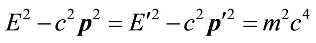 (9.2)
(9.2)
It seems quite clear that Equation (9.1) is invariant under the space-time inversion  and Equation (9.2) remains invariant under the mass inversion
  We believe that these two discrete symmetries are deeply rooted at the SR’s dynamics via its combination with QM and developing into RQM and QFT—the particle and its antiparticle are treated on equal footing and linked by the symmetry
  essentially. Hence we can perform a mass inversion on Equation (9.2) in each of two inertial frames with arbitrary relative velocity
  in the sense of
 , yielding:
 (9.3)
(9.3)
The invariance of Equation (9.2) under mass inversion as a whole reflects the experimental fact that particle and antiparticle are equally existing in nature even at the level of classical physics.
Example: The motion equation for a charged particle (say, electron with charge ) in the external electric and magnetic fields,
  and
and , is given by the Lorentz formula:
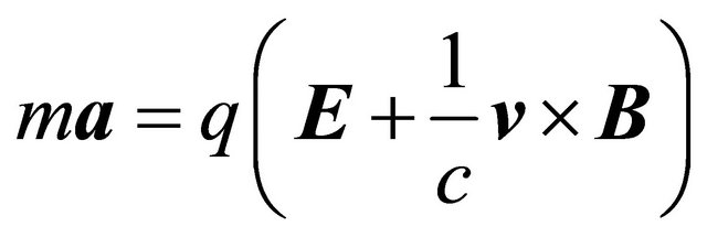 (9.4)
(9.4)
Then the operation of either  or
or
 on Equation (9.4) will realize the transformation from particle into its antiparticle (say, positron with charge
 ) with the acceleration change from
  as
as
 (9.5)
(9.5)
Based on what we learn from RQM (Sections III-V) as well as Equations (9.1)-(9.5), we may conjecture that for a classical theory being capable of treating matter and antimatter on an equal footing, it must be invariant under a mass inversion .
.
Notice that, however, Equation (9.4) (Equation (9.5)) is only valid for particle (antiparticle) moving at low speed, it must be modified to adapt to high-speed cases through the invariance of continuous Lorentz transformation. So we need “double checks” for testing a classical theory being really “relativistic” or not.
Let us restudy the theory of general relativity (GR). In a  metric, the Einstein field equation (EFE) reads (see, e.g. , Refs. [54-56])
 ,
,
 (9.6)
(9.6)
Of course, Equation (9.6) is covariant with respect to the Lorentz transformation. But could it withstand the test of mass inversion?
On the LHS of Equation (9.6), the Einstein tensor  contains no any mass and no charge as well. But on the RHS, the energy-momentum current density tensor
  is proportional to particle’s mass m and so changes its sign under an operation of
 . Hence as a whole, Equation (9.6) cannot remain invariant under the mass inversion. The reason seems rather clear that antimatter was not taking into account when GR was established in 1915. To modify EFE such that it can preserve the invariance of mass inversion, in 2004, one of us (Ni) proposed to add another term with
  for antimatter, yielding [27]
 (9.7)
(9.7)
which remains invariant under a mass inversion since:
 (9.8)
(9.8)
In a weak-field (or the post-Newtonian) approximation, this modified EFE, MEFE, Equation (9.7), will lead to modified Newton gravitational law as
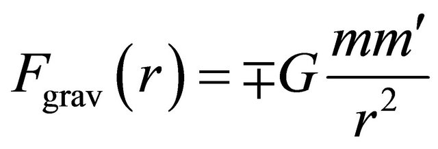 (9.9)
(9.9)
where the “ ” sign means attractive force between
  and
and  being both matter or antimatter whereas the “+” sign means repulsive force between
  and
and  (both positive) if one of them is antimatter.
If we define the “gravitational mass” for matter and antimatter separately
 (9.10)
Then Equation (9.9) can be recast into one equation
 (9.11)
which bears a close resemblance to the Coulomb law in classical electrodynamics (CED)
 (9.12)
In 1986, within the framework of classical field theory (CFT) plus some assumptions, Jagannathan and Singh derived the potential energy of two static point sources as [57]
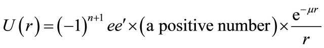 (9.13)
where  and
and  are spin and mass of the mediating field,
  is the “charge” of the source. For CED,
  whereas
  for gravitational field (
 in both cases). So Equation (9.13) is in conformity with Equations (9.11) and (9.12) for the case of “like sources” (with
 ) [57], where the case for “unlike sources”
  hadn’t been discussed. Here Equation (9.11) has been generalized to the case for “unlike sources”, but at a price that the “equivalence principle” in GR ceases to be valid when matter and antimatter coexist as shown by Equation (9.10).
In 2011, the antigravity between matter and antimatter was also claimed by Villata in Ref.[58], where the argument seems different from that explained above. But theory is theory, only fact will have the final say. So we are anxiously waiting for the outcome from the AEGIS experiment [59] (at CERN), which is designed to compare the Earth gravitational acceleration on hydrogen and antihydrogen atoms.
10. Summary
1) Being the combination of SR and QM, RQM is capable of dealing with particle and antiparticle on an equal footing. As long as we admit that the antiparticle’s momentum and energy operators should be 
and  versus
  and
and  for particle, it can be proved that the “negative-energy” WF
  of particle corresponds to a “positive-energy” WF
  of antiparticle precisely.
2) In general, an equation in RQM always has a discrete symmetry  which shows up as a transformation between a particle’s WF
  and its antiparticle’s WF
 :
: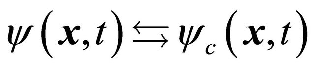 . For a free particle, it simply means
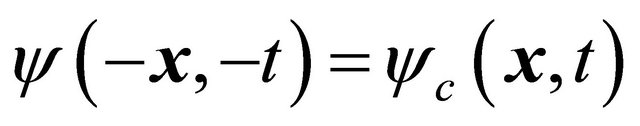 . This is in conformity with the “strong reflection” in QFT invented by Pauli and Lüders, showing that the intrinsic property of a particle cannot be detached from the space-time.
3) Following Feshbach-Villars’ deep insight, we are able to divide each and every WF  in RQM into two parts,
 . Then the above symmetry is further rigorously expressed by an invariance of motion equation in RQM through the transformations
  and
and  under either the space-time inversion
 or a mass inversion
 . Since
  in
in  whereas
  in
in , we may name
  as the (dominant) hidden particle field in
  while
while  the (subordinate) hidden antiparticle field in
 . In this way, both the “probability density”
  for a particle and
  for an antiparticle can be proved to be positive definite. Now we may say that the RQM is ensured to be self-consistent and can be regarded as a sound basis for QFT.
4) All kinematical effects in SR can be ascribed to the enhancement of the magnitude of  field in a particle’s WF accompanying with the increase of particle’s velocity.
5) As proved for Dirac particle with spin, the helicity of a particle is just opposite to that of its antiparticle under a space-time (or mass) inversion. Therefore, the experimental tests for the CPT invariance should include not only the equal mass and lifetime of particle versus antiparticle, but also the following fact: A particle and its antiparticle with opposite helicities must coexist in nature with no exception. A prominent example is the neutrino —A neutrino  (antineutrino
 ) is permanently lefthanded (right-handed) polarized whereas the fact that no
  exists in nature must means no
  as well (as verified by the GGS experiment [53]). See also Section VII.
6. Based on the invariance of space-time inversion or mass inversion (at the level of RQM) and the latter’s generalization to the classical physics, we tentatively discuss some interesting problems in today’s physics, including the prediction of antigravity between matter and antimatter, as well as the reason why we believe neutrinos are likely the tachyons.
11. Acknowledgements
We thank E. Bodegom, T. Chang, Y. X. Chen, T. P. Cheng, X. X. Dai, G. Tananbaum, V. Dvoeglazov, Y. Q. Gu, F. Han, J. Jiao, A. Kellerbauer, T. C. Kerrigan, A. Khalil, R. Konenkamp, D. X. Kong, J. S. Leung, P. T. Leung, Q. G. Lin, S. Y. Lou, D. Lu, Z. Q. Ma, D. Mitchell, E. J. Sanchez, Z. Y. Shen, Z. Q. Shi, P. Smejtek, X. T. Song, R. K. Su, G. Tananbaum Y. S. Wang, Z. M. Xu, X. Xue, J. Yan, F. J. Yang, J. F. Yang, R. H. Yu, Y. D. Zhang and W. M. Zhou for encouragement, collaborations and helpful discussions.
Appendix: Klein Paradox for Klein-Gordon Equation and Dirac Equation
We will discuss the Klein paradox [60] for both KG equation and Dirac equation based on Sections III and V, without resorting to the “hole” theory.
AI: Klein Paradox for KG Equation
Consider that a KG particle moves along  axis in onedimensional space and hits a step potential
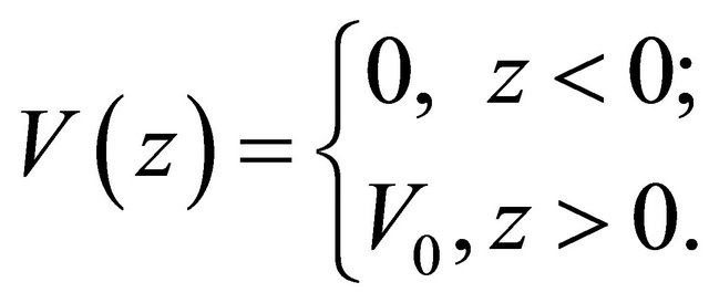 (A.1)
(A.1)
Its incident WF with momentum  and energy
  reads
reads
 (A.2)
(A.2)
If , we expect that the particle wave will be partly reflected at
  with WF
  and another transmitted wave
  emerged at
 :
:
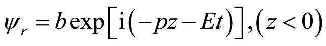 (A.3)
(A.3)
 (A.4)
(A.4)
with . See Figure 1(a).
Two continuity conditions for WFs and their space derivatives at the boundary  give two simple equations
 (A.5)
(A.5)
The Klein paradox happens when  because the momentum
 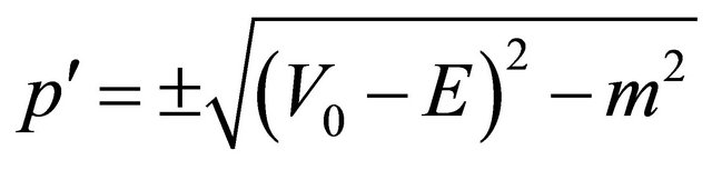 is real again and the reflectivity
  of incident wave reads
 (A.6)
(A.6)
(See Ref. [18] or  9.4 in Ref. [25], where discussions are not complete and need to be complemented and corrected here). Because the kinetic energy
  at
at  is negative:
 , what does it mean? Does the particle still remain as a particle?
As discussed in Section III, for a KG particle (or its antiparticle), two criterions must be held: its probability density ρ (or ) must be positive and its probability current density
  (or
(or ) must be in the same direction of its momentum
  (or
(or ).
).
See Figure 1(b), after making a shift in the energy scale, i.e., basing on the new vacuum at  region, we redefine a WF
  (which is actually the WF in the “interaction picture”,
 )
)
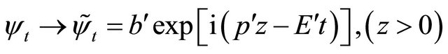 (A.7)
(A.7)
 . From now on we will replace KG WF
  by
by  and
and  according to Equation (3.26), if
  still describes a “particle”, whose probability density
  should be evaluated by Equation (27) with
 yielding:
 (A.8)
(A.8)
And its probability current density  should be given by Equation (3.12), yielding:
 (A.9)
(A.9)
Equation (A.8) is certainly not allowed. So to consider a “particle” with momentum  moving to the right makes no sense. Instead, we should consider
  (which also makes no sense for a particle due to the boundary condition) and regard
  as an antiparticle’s WF by rewriting it as:
 (A.10)
Now using Equation (2.18) we see that Equation (A.10) does describe an antiparticle with momentum
 and energy
 . In the mean time, from the antiparticle’s point of view (i.e., with
 ), the potential becomes
  (comparing Equation (2.21) with Equation (A.10) as shown by Figure 1(c).
It is easy to see from Equations (3.30), (3.31) and (A.10) that
 (A.11)
So the reflectivity, Equation (A.6), should be fixed as:
 (A.12)
And the transmission coefficient can also be predicted as:
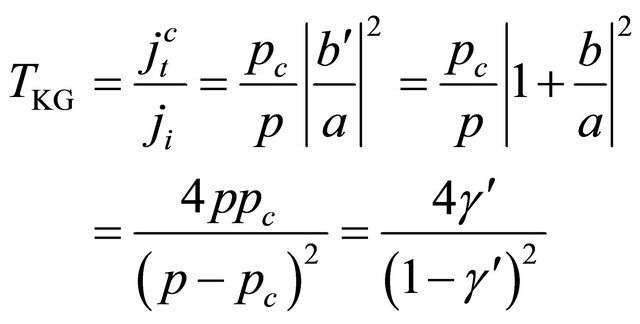 (A.13)
 (A.14)
The variation of  seems very interesting:
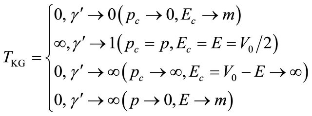 (A.15)
Above equations show us that the incident KG particle triggers a process of “pair creation” occurring at , creating new particles moving to the left side (to join the reflected incident particle) so enhancing the reflectivity
  and new antiparticles (with equal number of new particles) moving to the right.
To our understanding, this is not a stationary state problem for a single particle, but a nonstationary creation process of many particle-antiparticle system. It is amazing to see the Klein paradox in KG equation being capable of giving some prediction for such kind of process at the level of RQM. Further investigations are needed both theoretically and experimentally.10
AII: Klein Paradox for Dirac Equation
Beginning from Klein [60], many authors e.g. Greiner et al. [61,62], have studied this topic. We will join them by using the similar approach like that for KG equation discussed above.
Based on similar picture shown in Figure 1, now we have three Dirac WFs under the condition :
:
 (A.16)
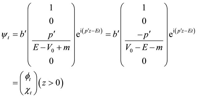
(A.17)
where . Unlike Equation (A.8)
for KG equation, the probability density for Dirac WF  is positive definite (see Equation (5.16))
 (A.18)
Hence we will rely on two criterions: First, the probability current density and momentum must be in the same direction for either a particle or antiparticle. For  and
and , their probability current density are

(A.19)
as expected. However, for , we meet difficulty similar to that in Equation (A.9)
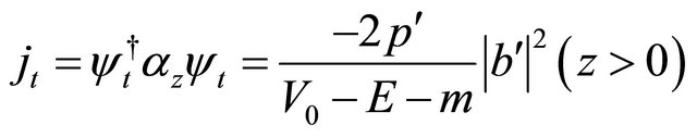 (A.20)
the direction of  is always opposite to that of
 ! The second criterion is: while
  for particle, we must have
  for antiparticle. Now in
  (or
(or
 ),
),  (or
(or ), but the situation in
is dramatically changed, the existence of  renders
 !
!
The above two criterions, together with the experience in KG equation, prompt us to choose  and regard
  as an antiparticle’s WF. So we rewrite:
 (A.21a)
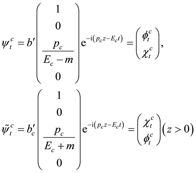 (A.21b)
where  (with new normalization constant
 replacing
 ) describes an antiparticle with momentum
 , energy
 and
and . Using Equation (5.17) we find
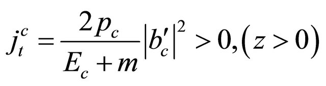 (A.22)
as expected. Now it is easy to match Dirac WFs at the boundary , (
, (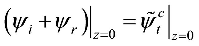 , yielding11
 (A.23)
where . The reflectivity
  and transmission coefficient
  follow from Equations (A.19) and (A.22) as:
 (A.24)
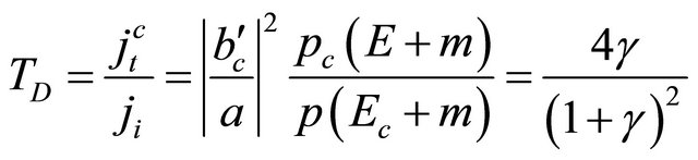 (A.25)
 (A.26)
where
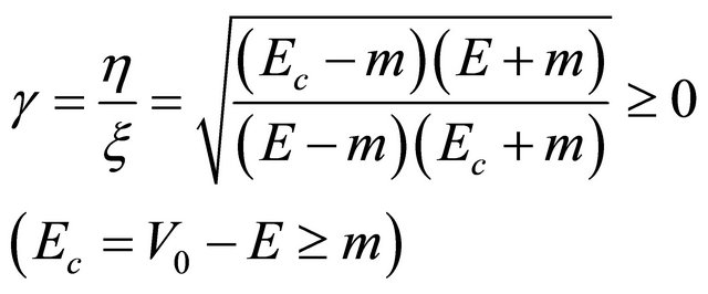 (A.27)
and
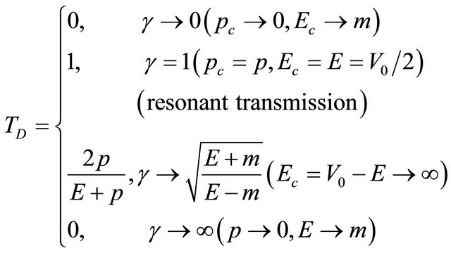 (A.28)
The variation of  bears some resemblance to Equation (A.15) for KG equation but shows striking difference due to sharp contrast between Equations (A.24)- (A.28) and Equations (A.12)-(A.15).
To our understanding, in the above Klein paradox for Dirac equation, there is no “pair creation” process occurring at the boundary . The paradox just amounts to a steady transmission of particle’s wave
  into a high potential barrier
  at
at  region where
  shows up as an antiparticle’s WF propagating to the right. In some sense, the existence of a potential barrier
  plays a “magic” role of transforming the particle into its antiparticle. Because the probability densities of both particle and antiparticle are positive definite, the total probability can be normalized over the entire space like that for one particle case:
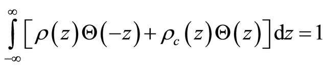 (A.29)
( is the Heaviside function) and the probability current density remains continuous at the boundary
 . In other words, the continuity equation holds in the whole space just like what happens in a one-particle stationary state.
It is interesting to compare our result with that in Refs. [61] and [62]. In Ref. [61], Equations (13.24)-(13.28) are essentially the same as ours. But the argument there for choosing  in Equation (13.23) is based on the criterion of the group velocity
  being positive (for the transmitted wave packet moving toward
 ). And the
  is stemming from Equation (13.16) which is essentially the probability current density in our Equations (A.21)-(A.22).
However, the author in Ref. [61] also considered the other choice  in an example (pp. 265-267 in [61]) based on the hole theory, ending up with the prediction as:
 (A.30)
where
 (A.31)
The argument for the validity of his Equations (A.30)- (A.31) is based on the hole theory (see also section 5.2 in Ref. [62]), saying that once , there would be an overlap between the occupied negative continuum for
  and the empty positive continuum for
 , providing a mechanism for electron-positron pair creation if the “hole” at
  can be identified with a positron. We doubt the “hole” theory seriously because there are only two electrons (with opposite spin orientations) staying at each energy level in the negative continuum. So it seems that there is no abundant source for electrons and “holes” to account for the huge value of
  in Equation (A.30).
Fortunately, we learn from section 10.7 in Ref. [62] that if the Klein paradox in Dirac equation is treated at the level of QFT, their result turns out to be the same form as our Equations (A.24)-(A.28), rather than Equations (A.30) and (A.31).
NOTES
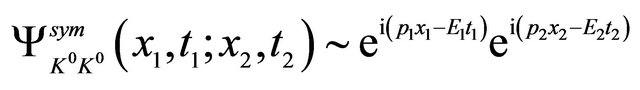 (2.14b)
which can be calculated from  with two terms. The squares of WF’s amplitude reproduces the
  in Equation (2.12).
2Please see the derivation of Equations (2.20) and (2.21) from the quantum field theory (QFT) at the end of Section VI.
3Interestingly, if ignoring the coupling between  and
and  and
and  in Equation (25), they satisfy respectively the “two equations” written down by Schrödinger in his 6th paper in 1926, titled “Quantisation as a problem of proper values (Part IV)” (Annalen der Physik Vol. 81, No. 4, 1926, p. 104) when he invented NRQM in the form of wave mechanics.
4Here m always refers to the “rest mass” also the “inertial mass” for a particle or its antiparticle, see the excellent paper by Okun in Ref. [33].
5Some pictures of numerical calculation are shown in Ref. [35] and section 9.5C at Ref. [25], where an error in Equation (9.5.26) is corrected here.
6The reason why we use  instead of
  will be clear in Equations (5.12)-(5.15). Actually, we emphasize Dirac equation as a coupling equation of two two-component spinors, Equation (3), rather than merely a four-component spinor equation.
7
8The wonderful experiment by Wu et al. [6] reveals the decay configuration of a polarized neutron bearing a strong resemblance to a “comet” with its “head” oriented along neutron’s spin parallel to  axis in space (note that a static neutron has no helicity
 , see [45]) while its “tail” composed of emitted
  and
and . So it was expected intuitively that [39] if one pushes the “comet” along its “head”’s direction, it (suddenly has a helicity
  and) will be relatively more stable than it is pushed along its “tail” (when it has
 ). That’s what Equation (7.1) means and why the use of “spin state” fails to get it right.
9We had discarded the solution of  in Equations (A.7)-(A.9) as a particle. However, if we consider
  for an antiparticle, then similar to Equations (A.10) and (A.11), we would get
  but both
  and
and  are negative, meaning that the antiparticle is coming from
 , not in accordance with our boundary condition. So the case of
  should be abandoned either as a particle or as an antiparticle.
10We find from the Google search that R. G. Winter in 1958 had written a paper titled “Klein paradox for the Klein-Gordon equation” and reached basically the same result as ours. So he was the first author dealing with this problem. Regrettably, it seems that his paper had never been published on some journal.
11Equation (A.23) means that the large (small) component of spinor is connected with large (small) component at both sides of . However, if instead of
 , the
, the  is used directly with its first (small) component being connected with the first (large) components of
  and
and , it would lead to a different expression of Equation (A.27):
 , which is just the
  (
( and
and  make no difference in the result of, say, Equations (A.24) and (A.25)) defined by Equation (8) on page 266 of Ref. [61] (see Equation (A31) below) or that by Equation (5.36) in Ref. [62]