1. INTRODUCTION
Among nature’s oscillators, the lunar tide is a wellunderstood familiar example. The sea level rises and falls with a period of about 12 hours, which is produced by the gravitational interaction of the moon circling the Earth. Another example is the diurnal atmospheric tide, which is produced by variable solar heating. Generated by external time dependent forcing, the tides are not autonomous oscillators. Oscillations that are forced by a time dependent source can be understood in terms of a linear system. Take n linear equations with n unknowns, A(n, n)·X(n) = S(n), A the square matrix of terms that account for dissipation, X the unknown linear column vector, and S the source vector. With X(n) = A−1(n, n)·S(n), A−1 the inverse matrix, it follows that an oscillation X ≠ 0 is produced with a source S ≠ 0 (Finite differencing produces the matrix elements for A to obtain a solution for a system of linear differential equations). In space physics, there is a large scientific body of literature featuring linear mathematical models that can generate and reproduce a variety of observed oscillations applying known excitation sources.
The above linear analysis demonstrates, with X(n) = A−1(n, n)·S(n), that for S = 0, X = 0. This means that without an external time dependent source, a linear system cannot produce an oscillation. Autonomous oscillators must be nonlinear—and a familiar example of such an oscillator is the pendulum clock. Once initiated, the clock continues oscillating at the resonance frequency that is determined by the length of the pendulum. The external source for the clock is the steady force of the weight pulling on the drive chain that activates the escapement wheel. With sufficient energy from the suspended weights to overcome friction, the escapement mechanism provides the impulse/nonlinearity that keeps the pendulum oscillating, as illustrated in Figure 1.
In mathematical terms, the variables (x, y) interact in a nonlinear system, like a1·xy + b1·xy = s1, a2·xy + b2·xy = s2, or for example a1·x2 + b1·y3 = s1, a2·x2 + b2·y3 = s2, where a12 and b12 account for dissipation such as friction, and s1, s2 are external sources that would be zero for the mechanical clock. A simple example of nonlinear interaction is illustrated with the temperature feedback of snow. In winter at high latitudes, as it gets colder, the precipitation turns into snow. White snowflakes, covering the ground, reflect incoming solar radiation to make it still colder. The interaction between diminishing radiation and resulting formation of ice crystals, two variables of climate change, say x, y, produce the nonlinear term, xy, that accelerates cooling. Another example of climate change is the melting of glaciers due to CO2-induced global warming. As the glaciers melt, the dark surface gets exposed and absorbs more solar radiation to acelerate the warming. Emptying a bottle with fluid would

Figure 1. In the mechanical clock, the escapement mechanism produces the impulse/nonlinearity that generates the oscillation without external time dependent source. Illustrated are the impulse sequence and broadband frequency sequence, which produce the pendulum oscillation with resonance frequency.
be a hands-on experiment demonstrating a nonlinear oscillation. The fluid pouring out, with sufficient speed, is compressed in the bottleneck. The resulting increase in pressure caused by the flow, a nonlinear feedback, slows down the flow to produce a glugging oscillation.
[1] reviewed the properties of observed fluid dynamical autonomous oscillators in space physics, foremost the quasi-biennial oscillation in the Earth’s atmosphere with a period of about two years, and the 22-year oscillation of the solar dynamo magnetic field. The oscillations have been simulated in numerical models without external time dependent source, and in Section 2 we summarize the results. Specifically, we shall discuss the nonlinearities involved in generating the oscillations, and the processes that produce the periodicities.
Stretch-activation of muscle contraction is the mechanism that produces the high frequency oscillation of autonomous insect flight, briefly discussed in Section 3. The same mechanism is also invoked to explain the functioning of the cardiac muscle. In Section 4, we present a tutorial review of the cardio-vascular system, heart anatomy, and muscle cell physiology, leading up to Starling’s Law of the Heart, which supports our notion that the human heart is also a nonlinear oscillator. In Section 5, we offer a broad perspective of the tenuous links between the modeled fluid dynamical oscillators and the human heart physiology.
2. FLUID-DYNAMICAL OSCILLATORS
In space physics, like in other areas of environmental science, mathematical models have been widely used to provide a physical understanding of the observations. Mentioned in the introduction, a large number of phenomena can be understood in terms of linear systems, like the diurnal atmospheric tide that is produced by variable solar heating. But there is no such external time dependent source known, which could produce the observed quasi-biennial oscillation in the atmosphere or the 22-year oscillation of the solar magnetic field. Numerical models generate the oscillations through nonlinear interactions that produce periodicities determined by the internal dynamical properties of the fluids.
2.1. Quasi-Biennial Oscillation (QBO)
In the zonal circulation of the terrestrial stratosphere at low latitudes, the quasi-biennial oscillation (QBO) dominates, and [2] presented a comprehensive review of the observations and physical mechanisms that generate the oscillation. Observed with satellites and ground-based measurements, the wind velocities vary between eastward and westward regimes that propagate down and have periods averaging approximately 28 months. Since its discovery more than 40 years ago, research has shown that the QBO plays an important role in a multitude of processes that affect the climate, as in the transmission of solar activity signatures and modulation of atmospheric tides for example. In the spirit of the subject matter of the present paper, we consider the QBO isolated from interactions with other atmospheric oscillations and focus on the fundamental processes that generate the QBO.
In a seminal paper published in 1968, [3] demonstrated that the QBO can be generated with planetary waves, and their theory was confirmed in numerous modeling studies. Subsequent studies showed that the QBO could also be reproduced with parameterized gravity waves (GW) [4,5], and this is now well accepted [2]. [3] considered the QBO being driven by the 6-month semi-annual oscillation (SAO) generated by solar heating. But [6] subsequently concluded that the SAO was not essential for generating the QBO, and this was confirmed in a modeling study [7].
From that paper, we present in Figure 2 computer solutions produced with the Numerical Spectral Model [4,8], which incorporates the Doppler Spread Parameterization [9,10] that provides the GW momentum source and associated eddy diffusivity/viscosity. Applying factor of two different diffusion or dissipation rates, QBO-like oscillations are produced with periods of about 33 and 17 months (Figures 2(a) and (b), respectively), which differ in amplitude by about a factor of two. The numerical results were generated for perpetual equinox, without time dependent solar heating. Without external time dependent source, the excitation mechanism cannot be linear, as demonstrated in Section 1. A nonlinear process must be involved in generating the oscillations.
The nonlinearity is displayed in Figure 3, which shows the zonal winds, U, and the accompanying GW momentum source, MS, varying with altitude. Discussed by [1,7], the positive nonlinear feedback associated with critical level of wave absorption produces a MS with sharp peaks near vertical wind shears, dU/dr. Considering the wind oscillation of the QBO, varying with frequency ω, the nonlinear part of the MS, to first order, can
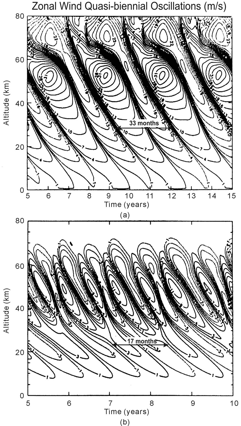
Figure 2. Altitude contour plots of equatorial zonal winds, positive eastward and negative westward. The winds were derived with diffusion/dissipation rates a factor of 2 larger in (b) than in (a). The resulting oscillation periods and amplitudes decrease with increasing dissipation rates; they are a factor of 2 smaller in (b) than in (a). A constant gravity wave (GW) flux provided the energy for the momentum source that generated the QBO-like oscillations. Figure taken from [7].
be written in the approximate form [dU(ω,r)/dr]3, of odd power. With complex notation, a source in the form [Exp(iωt)]3 produces the term with Exp[i(ω + ω + ω)t] for the higher order frequency, 3ω. Such a nonlinear source also generates Exp[i(ω + ω − ω)t] for the fundamental frequency ω, which maintains the oscillation.
2.2. Bimonthly Oscillation (BMO)
Zonal-mean oscillations with periods around 2 months have been seen in ground based and satellite wind measurements in the Earth atmosphere [12-14]. The Numerical Spectral Model generates such oscillations
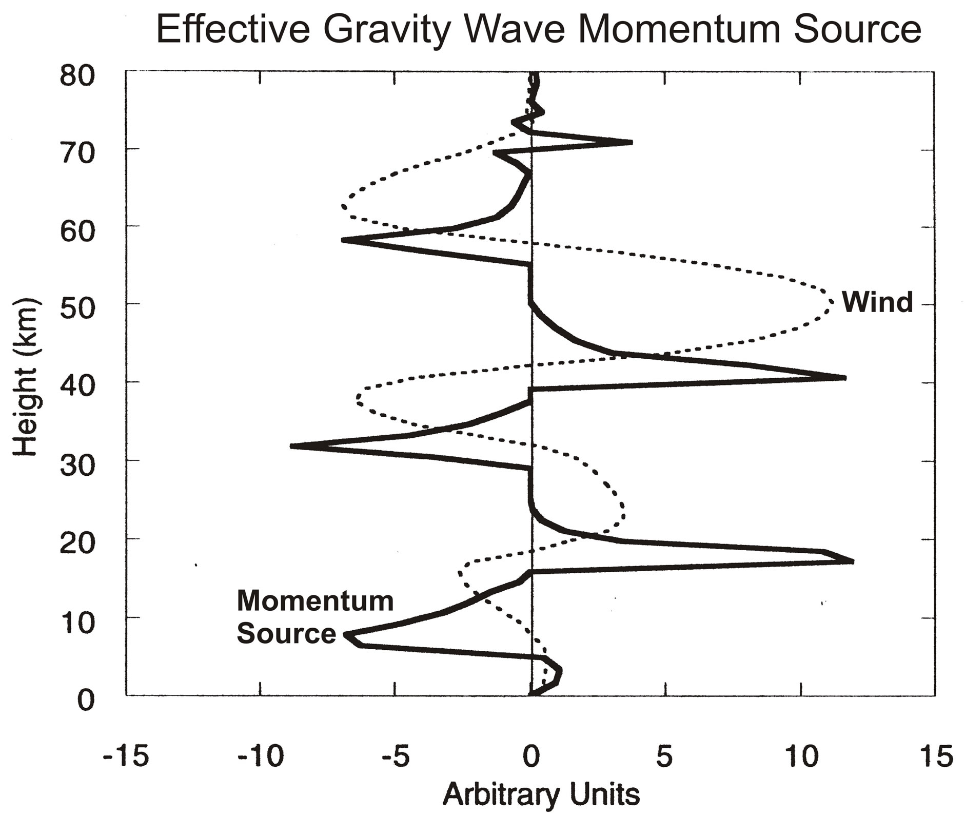
Figure 3. Snapshots are shown of zonal winds, and effective GW momentum source that generates the oscillations in Figure 2(b). The peak momentum source occurs near the maximum vertical velocity gradient; it varies in phase with the gradient and is strongly nonlinear. Figure taken from [11].
[15], and numerical experiments show that they are not produced when the gravity waves (GW) propagating north/south are turned off. In Figure 4(a), a computer solution is presented from that paper, which is produced only with the meridional (north/south) GW momentum source. Regular bimonthly oscillations (BMO) are generated with a period of about 2 months, which resemble the quasi-biennial oscillation (QBO) above discussed.
The similarity between the BMO and QBO is also evident in Figure 4(b), where meridional winds, V, are presented together with the associated momentum source. Like the GW source of the QBO in Figure 3, the momentum source in Figure 4(b) is sharply peaked near meridional wind shears. Discussed in Section 2.1, this impulsive momentum source can be viewed approximately as a nonlinear function of the velocity field, which has the character, [dV(ω,r)/dr]3. Such a non-linearity can generate an oscillation without external time-dependent forcing. Like the QBO, the meridional BMO can be understood as a nonlinear oscillator.
Like the QBO, the BMO is dissipated by viscosity. But unlike the zonal winds of the QBO, the meridional winds of the BMO produce pressure variations that counteract, and dampen, the winds to produce a shorter dissipative time constant. This additional thermodynamic feedback explains why the period of the BMO is much shorter than that of the QBO. In both cases, the oscillation periods are determined by the dissipation rates.
2.3. Solar Dynamo
The solar magnetic field is observed varying with a period of about 22 years. During periods of enhanced
 (a) (b)
Figure 4. (a) Meridional wind oscillations with periods of about 2 months. (b) Snapshots of normalized winds with momentum source that produces sharp peaks near vertical wind shears, similar to Figure 3. Figure taken from [15].
magnetic fields, irrespective of polarity, sunspots form around the equator that are associated with enhanced solar radiation. The resulting 11-year cycle of solar activity produces variations that strongly depend on the wavelength of the emitted radiation. At lower altitudes in the atmosphere near the ground, the solar cycle effect is relatively small. But with increasing altitude, the effect increases due to the shorter wavelength ultraviolet radiation that is absorbed, and above 150 km, the medium of artificial satellites, the radiative input can vary by as much as a factor of 2 during the solar cycle. The solar cycle and its periodicity are variable, and empirical models that employ the observed precursor polar magnetic field during the minimum have been very successful in predicting the magnitude and duration of the solar maximum [16].
Pars pro toto, we refer here to the magneto hydro-dynamic (MHD) model of [17]. [17] generate the solar oscillation with a zonal-mean magnetic field model, which produces the solar oscillation shown in Figure 5. In this model, the poloidal (radial) magnetic field is wound up by solar differential rotation to produce a toroidal (longitudinal) field in the tachocline below the convective envelope. The buoyant toroidal field emerges at the top of the convection region to form sunspots. In that process, the Coriolis force is twisting the toroidal field to regenerate the poloidal field.
[17] artificially add in their equation for the poloidal magnetic field a nonlinear term presented here in a Taylor series expansion with variable Bf(rc,θ,t), where Bf represents the toroidal magnetic field, (r,θ) are spherical polar coordinates (rc, for the tachocline region), and Bo is taken to be constant,
 (1)
(1)
 (a) (b)
Figure 5.Shown is the radial magnetic field varying with a period of 20 years. Solid (dashed) contours correspond to positive (negative) magnetic fields, which are spaced logarithmically, with three contours covering a decade of field strength. Figure is taken from the MHD dynamo model of [17].
The nonlinear source terms of Eq.1 have the property that they are of odd (e.g., 3rd) power, a similar nonlinearity also appears in the classical dynamo model of [18]. In dynamo models, the nonlinear terms have the character of the momentum source (Figure 3) that generates the quasi-biennial oscillation (QBO). The QBO and solar dynamo have furthermore in common that the oscillation periods are determined by the dissipation rates. For the QBO, it is the eddy viscosity; and in the MHD model of [17], the magnitude of the dissipating meridional circulation mainly controls the period of the solar cycle.
3. INSECT FLIGHT
Insect flight is an outstanding example of autonomous oscillation, and the muscle physiology involved has served as a model for understanding the human heart.
In an advanced class of insects, wing frequencies as large as 1000 Hz are produced, which are determined by the inertia of the wings and far exceed the frequency capacity of the animals’ neural system [19]. This autonomous flight mechanism is produced by stretchactivation of muscle contraction [20,21], which is also important for the mammalian heart. Insect flight is very demanding energetically, and stretch-activation proves to be well suited to match the wing frequency to the aerodynamic load, making the insect “one of the most successful animals that have conquered air” [22]. In this fascinating class of insects, the flight muscles are integrated into the animal’s elastic thorax (Figure 6), changing its shape. They are therefore referred to as indirect flight muscles. The pair of dorsoventral muscles (Figure 6(a)) contract and pull the tergal plate at the back of the insect down, which causes the hinged wings to flip upwards. The longitudinal muscles (Figure 6(b)) run horizontally and compress the thorax from front to back, which causes the thorax to bow upwards and make the wings flip downwards. These antagonistic pairs of flight

Figure 6. Insect cross-sections illustrate (a) contraction by the dorsoventral muscles that pull the tergal plate down to make the hinged wings move up, and (b) contraction of the longitudinal muscles that push the tergal plate up and the wings down. Figures taken from [23].
muscles work in tandem through stretch-activation. When the dorsoventral muscle contracts to lift the wings up (Figure 6(a)), the longitudinal muscle is stretched to activate its contraction that pulls the wings down (Figure 6(b)), and vice versa. The two antagonistic muscles alternately stretch and contract. Stretch activates the muscle contractions that force the wings up and down to produce the high frequency oscillation of autonomous insect flight. Nerve impulses command the insect flight but at a rate much slower than the wing oscillation; hence it is referred to as asynchronous flight.
4. HUMAN HEART
A tutorial review is presented of the human heart function, which provides the framework for the notion that the autonomous heart can be understood as a nonlinear oscillator.
4.1. Heart Physiology
In the cardiovascular system [24], illustrated in Figure 7, the human heart exchanges blood with the pulmonary and systemic circuits that complement each other. Oxygen-rich and CO2-poor blood, returning from the lungs in veins, is pumped in arteries by the left side of the heart to the tissue cells of the human body. The returning blood in veins, oxygen-poor and CO2-rich, is pumped in arteries by the right heart into the lungs that pick up oxygen and shed CO2.
Figure 8 illustrates the human heart anatomy. The heart functions through the interplay between the receiving chambers, the atria, and the main pumping chambers,