Solid Boundary as Energy Source and Sink in a Dry Granular Dense Flow: A Comparison between Two Turbulent Closure Models ()
1. Introduction
Dry granular dense flows are continuous motions of a large amount of discrete solid particles with interstitial space filled by a gas, moving with slow to moderate speed. The grain-grain interaction, in contrast to creeping or rapid flows, results from ong-term enduring frictional contact and sliding, and short-term instantaneous inelastic collision [1] - [4] . Two-fold grain-grain interactions induce fluctuations on the field quantities at the macroscopic level, a phenomenon similar to turbulent motion of Newtonian fluids with two distinctions: 1) it emerges from grain-grain interactions, in contrast to those resulted from incoming flow instability, instability in transition region, or flow geometry in Newtonian fluids; and 2) it emerges at slow speed, in contrast to those in Newtonian fluids which are strongly velocity-dependent, characterized by the critical Reynolds’ number [5] [6] .
Solid boundary has been demonstrated to be an energy source and sink of the turbulent kinetic energy of the grains, and conventional no-slip condition of velocity is not valid [7] [8] . Whereas these influences were hardly accounted for in laminar flow formulations, e.g. [9] - [17] , they were not appropriately taken into account in the limiting turbulent flow formulations, e.g. [18] - [21] . Thus, the goal of the present study is to propose a ther- modynamically consistent turbulent closure model to account for these effects, with their influence on the mean and turbulent flow features. Specifically, a zero- and a first-order closure models are proposed, with the focus on the intercomparison of the roles played by the solid boundary, and the influence of velocity slip.
In the following sections, the mean balance equations, state space and entropy inequality are presented for two models. The closure relations are summarized as results from thermodynamic considerations of the first and second laws. Two closure models are applied to analyses of stationary gravitational flows down an inclined moving plane. While solutions of two models demonstrate a qualitative agreement with experimental outcomes in the mean porosity and velocity profiles, the distributions of the turbulent dissipation are similar to those of Newtonian fluids in turbulent boundary layer flows, with their vanishing and finite values obtained on the free surface by the zero- and first-order models, respectively. Increasing velocity slip near the inclined plane tends to enhance the turbulent dissipation nearby, resulting in larger mean porosity and turbulent kinetic energy near the free surface. While boundary as energy source and sink is apparent in the first-order model, its latter role is more obvious in the zero-order model.
2. Mean Balance Equations and Equilibrium Closure Relations
To account for the distribution of solid volume and its microstructural effect, the (solid) volume fraction , defined as the total solid volume divided by the volume of a granular representative volume element (RVE), is introduced, with its time evolution described by the Wilmánski model for dense flows [12] [22] . A dense flow is considered a rheological fluid, which must satisfy the basic laws of motion for continuum mechanics. Since in turbulent motion the field quantities experience fluctuations, with solutions random and unpredictable, their sta- tistically averaged values (e.g. Reynolds-averaging) should be defined and investigated. With these, the fol- lowing mean balance equations must be satisfied [5] [12] [23] [24]
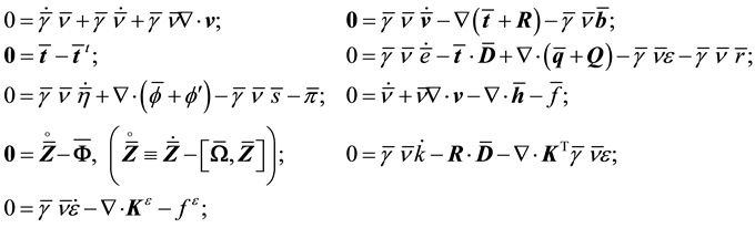
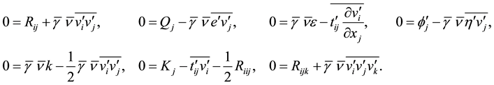
with the ergodic terms,
 (6)
(6)
The variables and parameters in (1)-(6) are defined in Table 1.
Equations (1)1.2, (2)1.2 and (3)1 are respectively the conventional mean balances of mass, linear momentum, angular momentum, internal energy and entropy for a continuum, with the mean density  decomposed into
 , and the symmetry of the mean Cauchy stress is required. Equation (3)2 is the Wilmánski model for
![]()
Table 1. Variables and parameters in the mean balance equations.
the time evolution of , Equation (4)1 is the phenomenological generalization of the Mohr-Coulomb model for the mean internal friction in a granular material at low energy and high-grain volume fraction [12] [25] [26] , while Equations (4)2 and (5) are the balances of turbulent kinetic energy and dissipation, respectively. They are included to denote the influence of the energy cascade from the mean flow scale toward the smallest (dissipation) scale in turbulent flows. In doing so, two turbulent closure models are constructed: Equations (1)-(4) apply for the zero-order model with the turbulent dissipation considered a closure relation, and Equations (1)-(5) apply for the first-order
  model, in which the time evolutions of the turbulent kinetic energy and dissipation are des- cribed independently and separately.
For the application of two models, the quantities
 (7)
(7)
are introduced as the primitive mean fields, with the superscripts 0 and 1 denoting the model specification, while the closure relations
 (8)
(8)
are constructed based on the state spaces given by
 (9)
(9)
with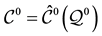 , and
, and , where
 ,
,  ,
,  ,
, ![]() ,
, ![]() ,
, ![]() , and
, and ![]() the Nabla operator. The quantity
the Nabla operator. The quantity ![]() is the material coldness, with
is the material coldness, with ![]() the granular coldness, a si- milar concept to granular temperature [20] [23] - [25] [27] [28] . While it is used to index both variations in tur- bulent kinetic energy and dissipation in the zero-order model, it is employed only for the variation in turbulent kinetic energy in the first-order model. The quantity
the granular coldness, a si- milar concept to granular temperature [20] [23] - [25] [27] [28] . While it is used to index both variations in tur- bulent kinetic energy and dissipation in the zero-order model, it is employed only for the variation in turbulent kinetic energy in the first-order model. The quantity ![]() is the value of
is the value of ![]() in the reference configuration, included due to its influence on flowing granular matter. In (9),
in the reference configuration, included due to its influence on flowing granular matter. In (9), ![]() ,
, ![]() ,
, ![]() ,
, ![]() ,
, ![]() and
and ![]() are for the ela- stic effect;
are for the ela- stic effect; ![]() and
and ![]() represent the temperature-dependence of physical properties,
represent the temperature-dependence of physical properties, ![]() with
with ![]() and
and ![]() with
with ![]() denote the influence of turbulent fluctuation, while
denote the influence of turbulent fluctuation, while ![]() and
and ![]() are for the viscous and rate- independent effect, respectively.
are for the viscous and rate- independent effect, respectively.
The forms of the closure relations are reduced by the second law of thermodynamics, which is formulated here as the Müller-Liu entropy principle. In its local form, it represents the restriction that the mean entropy production must be non-negative, i.e.,![]() . A physically admissible process must si- multaneously satisfy this Equation, (1)-(2) and (3)
. A physically admissible process must si- multaneously satisfy this Equation, (1)-(2) and (3)![]() -(5). One can account for all these requirements by using the method of Lagrange multiplier, viz.,
-(5). One can account for all these requirements by using the method of Lagrange multiplier, viz.,
![]() (10)
(10)
with the mean balance equations appearing as constraints of the entropy inequality, and![]() ,
, ![]() ,
, ![]() ,
, ![]() ,
, ![]() ,
, ![]() ,
, ![]() ,
, ![]() the corresponding Lagrange multipliers.
the corresponding Lagrange multipliers.
Substituting (8) and (9) into (10) with the assumption of material isotropy and chain rule of differentiation, the corresponding restrictions on forms such as (8) have been defined elsewhere [23] [24] . They are expressions for ![]() and
and![]() ,
, ![]() and
and![]() , as well the dependence of the specific turbulent Helmholtz free energies
, as well the dependence of the specific turbulent Helmholtz free energies ![]() and
and![]() , defined by
, defined by ![]() and
and![]() , for the zero- and first- order models, respectively, viz.,
, for the zero- and first- order models, respectively, viz.,
![]() (11)
(11)
with![]() ,
, ![]() ,
, ![]() and
and![]() . The
. The
expressions of ![]() and
and![]() ,
, ![]() and
and![]() ,
, ![]() ,
, ![]() and
and![]() ,
, ![]() and
and![]() ,
, ![]() ,
,
![]() and
and ![]() at an thermodynamic equilibrium state denoted by the subscript
at an thermodynamic equilibrium state denoted by the subscript![]() , defined by
, defined by
![]() and
and ![]() in the zero- and first-order models, respectively, are given by
in the zero- and first-order models, respectively, are given by
![]()
where![]() . The variables
. The variables ![]() and
and ![]() stand for the turbulent thermodynamic and configurational
stand for the turbulent thermodynamic and configurational
pressures, respectively, viz.,
![]() (20)
(20)
for both models. Otherwise, for incompressible grains, ![]() is an independent field and can no longer be deter- mined by Equation (20)1; Equations (11)1, (18) and (19) are simplified to [12]
is an independent field and can no longer be deter- mined by Equation (20)1; Equations (11)1, (18) and (19) are simplified to [12]
![]() (21)
(21)
![]() (22)
(22)
![]() (23)
(23)
while (11)2-3 and (12)-(16) remain unchanged, with (17) reducing to![]() .
.
3. Closure Models
For isothermal flows with incompressible grains, we assume that![]() ,
, ![]() ,
, ![]() ,
, ![]() ,
, ![]() ,
, ![]() ,
, ![]() and
and ![]() may be decomposed according to
may be decomposed according to
![]() (24)
(24)
with![]() ; the superscript
; the superscript ![]() indicates dynamic response, which should vanish at thermodynamic equi- librium. Within a quasi-static theory, the dynamic responses are assumed to depend explicitly and linearly on the independent dynamic variables, respectively of the forms,
indicates dynamic response, which should vanish at thermodynamic equi- librium. Within a quasi-static theory, the dynamic responses are assumed to depend explicitly and linearly on the independent dynamic variables, respectively of the forms,
![]()
with ![]() -
-![]() ,
, ![]() and
and ![]() functions of
functions of![]() ;
;![]() ,
, ![]() ,
, ![]() and
and ![]() functions of
functions of![]() and the three invariants
and the three invariants ![]() of
of![]() . The functional dependences of
. The functional dependences of ![]() and
and ![]() are the same as above, with
are the same as above, with ![]() additionally included. We choose the material vis- cosities
additionally included. We choose the material vis- cosities ![]() and phenomenological (turbulent) viscosities
and phenomenological (turbulent) viscosities ![]() be given by [12] [16] [17] [26]
be given by [12] [16] [17] [26]
![]() (28)
(28)
with ![]() depending on the three invariants of
depending on the three invariants of![]() ;
;![]() , a positive constant;
, a positive constant; ![]() the mean vol- ume fraction corresponding to the possible most dense packing of the grains; and
the mean vol- ume fraction corresponding to the possible most dense packing of the grains; and ![]() the critical mean volume fraction at which shearing is decoupled from dilatation. Equation (28) asserts that the total stress is larger in turbulent than in laminar flows, and is justified for weak turbulent intensity [29] [30] .
the critical mean volume fraction at which shearing is decoupled from dilatation. Equation (28) asserts that the total stress is larger in turbulent than in laminar flows, and is justified for weak turbulent intensity [29] [30] .
For explicit expressions of![]() ,
, ![]() ,
, ![]() and
and![]() , the simplest form of the specific turbulent free energy is proposed following previous works by [12] [17] [26]
, the simplest form of the specific turbulent free energy is proposed following previous works by [12] [17] [26]
![]() (29)
(29)
with the plastic contribution confined within![]() . Equation (29) is justified for weak turbulent flows, and as- serts that smaller granular coldness results in smaller free energy [27] - [30] . A hypoplastic form for the mean production of mean internal friction is given by [31] [32]
. Equation (29) is justified for weak turbulent flows, and as- serts that smaller granular coldness results in smaller free energy [27] - [30] . A hypoplastic form for the mean production of mean internal friction is given by [31] [32]
![]() (30)
(30)
to account for rate-independent characteristics, in which![]() , the versor of
, the versor of![]() ;
;![]() , the deviator of
, the deviator of![]() ;
;![]() , and
, and ![]() a positive constant, relating to the internal friction and frictional angle in the critical state. The scalar functions
a positive constant, relating to the internal friction and frictional angle in the critical state. The scalar functions ![]() and
and ![]() are the stiffness and density factors, denoting strain harding/soft- ing and mean-pressure dependent bulk density, respectively.
are the stiffness and density factors, denoting strain harding/soft- ing and mean-pressure dependent bulk density, respectively.
The specific forms (28)-(30) are assigned for both models, for they are proposed based on experiments. With these, the closure relations of![]() ,
, ![]() ,
, ![]() ,
, ![]() ,
, ![]() ,
, ![]() ,
, ![]() ,
, ![]() ,
, ![]() and
and ![]() for an isochoric, isothermal flow with incompressible grains and weak turbulent intensity are given by
for an isochoric, isothermal flow with incompressible grains and weak turbulent intensity are given by
![]() (31)
(31)
![]() (32)
(32)
![]() (33)
(33)
![]() (34)
(34)
with![]() , where Cayley-Hamilton theorem, Truesdell’s equi-presence principle and the notations
, where Cayley-Hamilton theorem, Truesdell’s equi-presence principle and the notations
![]() (35)
(35)
are used. Substituting (20), (21), (30)-(34) into (1)-(5) yields the field equations for both models.
4. Inclined Gravity-Flow Problem
4.1. Field Equations and Boundary Conditions
Consider a fully-developed, isothermal, two-dimensional stationary turbulent shear flow down an inclined mov- ing plane, as shown in Figure 1. With this,
![]() (36)
(36)
and![]() ,
, ![]() ,
, ![]() , are assumed, with
, are assumed, with![]() ;
;![]() ,
, ![]() ,
, ![]() and
and ![]() the mean velocity component in the
the mean velocity component in the ![]() direction, the mean volume fraction, the granular coldness and the mean internal friction components, respectively; and
direction, the mean volume fraction, the granular coldness and the mean internal friction components, respectively; and ![]() applies for the first-order model.
applies for the first-order model.
The flow corresponds to the critical state, defined as the state in which ![]() and
and ![]() [33] [34] . Since in the critical state
[33] [34] . Since in the critical state ![]() is set to be unity, Equation (30) reduces to
is set to be unity, Equation (30) reduces to
![]() (37)
(37)
in which![]() , the value of
, the value of ![]() at the critical state; and
at the critical state; and ![]() the critical friction angle [34] . Since
the critical friction angle [34] . Since ![]() does not vanish in general, substituting (37) into (4)
does not vanish in general, substituting (37) into (4)![]() yields
yields
![]() (38)
(38)
with![]() . The only non-trivial solution of (38) is
. The only non-trivial solution of (38) is ![]() and
and![]() . Thus, Equation (4)1 is decoupled from other mean balance equations in both models. For further identification, a specific form of
. Thus, Equation (4)1 is decoupled from other mean balance equations in both models. For further identification, a specific form of ![]() is proposed by [35] [36]
is proposed by [35] [36]
![]()
Figure 1. Gravity-driven stationary flow down an inclined moving plane and the coordinate.
![]()
Table 2. Dimensionless parameters in the dimensionless field equations.
![]() (39)
(39)
with ![]() the minimum mean volume fraction. With these, the mean field equations reduce to
the minimum mean volume fraction. With these, the mean field equations reduce to
![]() (40)
(40)
![]() (41)
(41)
![]() (42)
(42)
![]() (43)
(43)
![]() (44)
(44)
for![]() ,
, ![]() ,
, ![]() and
and![]() , where Equations (40)-(42) apply for the zero-order model, and (40)-(41) and (43)-(44) apply for the first-order model.
, where Equations (40)-(42) apply for the zero-order model, and (40)-(41) and (43)-(44) apply for the first-order model.
Due to velocity slip, the grains on the solid plane may not assume the plane velocity. Velocity slip provides extra energy flux toward to, or away from the granular body, which is proportional to the square of the slip velocity and with the same direction of the momentum flux on the boundary [7] [8] . On the contrary, due to the experimental setup [37] , ![]() approaches a fixed value on the solid plane. Since experiment is carried out by discharging a constant mass flux on the plane, the flow thickness is fixed, and the shear force on the free surface is negligible due to the significant density difference between the granular body and air. Thus, the boundary conditions are given by
approaches a fixed value on the solid plane. Since experiment is carried out by discharging a constant mass flux on the plane, the flow thickness is fixed, and the shear force on the free surface is negligible due to the significant density difference between the granular body and air. Thus, the boundary conditions are given by
![]() (45)
(45)
with![]() ,
, ![]() and
and ![]() the boundary values on the inclined plane;
the boundary values on the inclined plane; ![]() the velocity of the solid plane;
the velocity of the solid plane; ![]() the grain velocity on the plane;
the grain velocity on the plane; ![]() and
and ![]() the coefficients relating respectively the contributions of the slip velocity
the coefficients relating respectively the contributions of the slip velocity ![]() to the boundary values of
to the boundary values of ![]() and
and![]() ; and
; and ![]() the flow thickness. The prescription of
the flow thickness. The prescription of ![]() on the plane applies only for the first-order model. In doing so, solid boundary as an energy source and sink is taken into account by prescribing the values of
on the plane applies only for the first-order model. In doing so, solid boundary as an energy source and sink is taken into account by prescribing the values of ![]() and
and ![]() separately in the first-order model, and by a fixed boundary value of
separately in the first-order model, and by a fixed boundary value of ![]() in the zero-order model. Nonvanishing
in the zero-order model. Nonvanishing ![]() and
and ![]() correspond to experimental ob- servations at vanishing slip velocity.
correspond to experimental ob- servations at vanishing slip velocity.
4.2. Nondimensionalization and Numerical Method
With the dimensionless parameters defined in Table 2, Equations (40)-(44) are recast respectively by
![]() (46)
(46)
![]() (47)
(47)
![]() (48)
(48)
![]() (49)
(49)
with the dimensionless boundary conditions,
![]() (50)
(50)
where![]() ,
, ![]() and
and![]() .
.
The two-point nonlinear BVPs (46)-(50) are solved numerically by means of the method of successive ap- proximation with under-relaxation scheme. For the implementation of numerical simulation, the values of![]() ,
, ![]() ,
, ![]() and
and ![]() are given by [12] [16] [35]
are given by [12] [16] [35]
![]() (51)
(51)
with fixed values of ![]() and
and![]() , motivated by experimental observations.
, motivated by experimental observations.
4.3. Numerical Results
As a parametric study, numerical simulations are carried out for variations in![]() ,
, ![]() and
and![]() , with
, with![]() ,
, ![]() ,
, ![]() ,
, ![]() ,
, ![]() and
and![]() . The inclined angle
. The inclined angle ![]() is chosen to match the experiments [37] .
is chosen to match the experiments [37] .
Figure 2 illustrates the profiles of ![]() (the mean porosity),
(the mean porosity), ![]() and the dimensionless turbulent kinetic energy and dissipation, in which
and the dimensionless turbulent kinetic energy and dissipation, in which ![]() indicated by the arrows, with the dashed lines representing laminar flow solutions [12] . Decreasing
indicated by the arrows, with the dashed lines representing laminar flow solutions [12] . Decreasing ![]() tends to increase velocity slip on the solid plane, resulting in more intensive friction near the solid plane with significant turbulent dissipation, as shown in Figure 2(f) and Figure 2(j) in both models. Due to velocity slip, the shearing generated by the plane is less efficiently transferred toward the granular body. The flow above the slip surface is dominated by gravity, in which the grains are moving with larger velocity in the reverse direction, as shown in Figure 2(d) and Figure 2(h). In this region, the grains are colliding with one another in a relatively free manner, resulting in larger mean porosity and di- mensionless turbulent kinetic energy, as shown in Figure 2(c) with Figure 2(g) and Figure 2(e) with Figure 2(i), respectively. The profiles of
tends to increase velocity slip on the solid plane, resulting in more intensive friction near the solid plane with significant turbulent dissipation, as shown in Figure 2(f) and Figure 2(j) in both models. Due to velocity slip, the shearing generated by the plane is less efficiently transferred toward the granular body. The flow above the slip surface is dominated by gravity, in which the grains are moving with larger velocity in the reverse direction, as shown in Figure 2(d) and Figure 2(h). In this region, the grains are colliding with one another in a relatively free manner, resulting in larger mean porosity and di- mensionless turbulent kinetic energy, as shown in Figure 2(c) with Figure 2(g) and Figure 2(e) with Figure 2(i), respectively. The profiles of ![]() and
and ![]() corresponding qualitatively to the experimental outcomes (see Figure 2(c) with Figure 2(g) with Figure 2(a), and Figure 2(d) and Figure 2(h) with Figure 2(b)). The nu- merical results approach better to the experimental measurements with smaller values of
corresponding qualitatively to the experimental outcomes (see Figure 2(c) with Figure 2(g) with Figure 2(a), and Figure 2(d) and Figure 2(h) with Figure 2(b)). The nu- merical results approach better to the experimental measurements with smaller values of ![]() in both models, resulted from the fact that velocity slip is identified near the solid plane in experiments. This finding suggests that the influence of velocity slip needs be taken into account for more accurate numerical prediction.
in both models, resulted from the fact that velocity slip is identified near the solid plane in experiments. This finding suggests that the influence of velocity slip needs be taken into account for more accurate numerical prediction.
The dimensionless turbulent dissipations, shown in Figure 2(f) and Figure 2(j), decrease from their ma- ximum values on the solid plane toward the minimum values on the free surface with an “exponential-like” tendency in variations in ![]() in both models. Although such a tendency is similar to that of Newtonian fluids in turbulent boundary layer flows [5] [6] , the first-order model is more justified, for finite turbulent dissipation is obtained on the free surface, where the turbulent kinetic energy is maximum (see Figure 2(e) and Figure 2(f)), in contrast to vanishing turbulent dissipation from the zero-order model (see Figure 2(i) and Figure 2(j)). This is due to that in the first-order model, the turbulent kinetic energy and dissipation are indexed separately by
in both models. Although such a tendency is similar to that of Newtonian fluids in turbulent boundary layer flows [5] [6] , the first-order model is more justified, for finite turbulent dissipation is obtained on the free surface, where the turbulent kinetic energy is maximum (see Figure 2(e) and Figure 2(f)), in contrast to vanishing turbulent dissipation from the zero-order model (see Figure 2(i) and Figure 2(j)). This is due to that in the first-order model, the turbulent kinetic energy and dissipation are indexed separately by ![]()
and![]() , respectively, whilst in the zero-order model,
, respectively, whilst in the zero-order model, ![]() is used as a direct measure of the turbulent kinetic energy and an indirect measure of the turbulent dissipation.
is used as a direct measure of the turbulent kinetic energy and an indirect measure of the turbulent dissipation.
Difference between two models can further be recognized by the profiles of![]() , as shown in Figure 2(d) and Figure 2(h). While in the zero-order model a “local” energy balance is imposed between the turbulent kinetic energy and dissipation, the influence of turbulent eddy evolution is accounted for in the first-order model, re- sulting in more efficient turbulent kinetic energy transfer across the flow. This leads to more efficient transfer of the mean shearing and stress power of the solid plane, giving rise to a discrepancy isn the lower and central regions, when compared with experimental outcomes and those from the zero-order model. It should not be concluded, however, that the first-order model is inaccurate, for the flows in experiments deviate only slightly from laminar flow. On the other hand, Figure 2(d) and Figure 2(h) demonstrate that the turbulent eddy evo- lution influences significantly on the mean flow characteristics, and need be taken into account when the turbulent intensity is not weak.
, as shown in Figure 2(d) and Figure 2(h). While in the zero-order model a “local” energy balance is imposed between the turbulent kinetic energy and dissipation, the influence of turbulent eddy evolution is accounted for in the first-order model, re- sulting in more efficient turbulent kinetic energy transfer across the flow. This leads to more efficient transfer of the mean shearing and stress power of the solid plane, giving rise to a discrepancy isn the lower and central regions, when compared with experimental outcomes and those from the zero-order model. It should not be concluded, however, that the first-order model is inaccurate, for the flows in experiments deviate only slightly from laminar flow. On the other hand, Figure 2(d) and Figure 2(h) demonstrate that the turbulent eddy evo- lution influences significantly on the mean flow characteristics, and need be taken into account when the turbulent intensity is not weak.
Numerical simulations have been carried out for variations in ![]() and the results are summarized in Figure 3, in which
and the results are summarized in Figure 3, in which ![]() indicated by the arrows. Increasing
indicated by the arrows. Increasing ![]() tends to enhance the energy flux from the solid plane toward granular body (boundary as energy source), yielding more intensive turbulent dissipation near the solid plane and near the free surface in the zero- and first-order models, respectively, as shown in Figure 3(d) and Figure 3(h). Since intensive turbulent kinetic energy induces intensive turbulent dissipation, as implied by Newtonian fluids characteristics, the first-order model is more justified than the zero-order model (see Figure 3(c) and Figure 3(d) with Figure 3(g) and Figure 3(h)). With the enhanced turbulent dissipation, the profiles of
tends to enhance the energy flux from the solid plane toward granular body (boundary as energy source), yielding more intensive turbulent dissipation near the solid plane and near the free surface in the zero- and first-order models, respectively, as shown in Figure 3(d) and Figure 3(h). Since intensive turbulent kinetic energy induces intensive turbulent dissipation, as implied by Newtonian fluids characteristics, the first-order model is more justified than the zero-order model (see Figure 3(c) and Figure 3(d) with Figure 3(g) and Figure 3(h)). With the enhanced turbulent dissipation, the profiles of ![]() and
and ![]() shown in Figure 3(a), Figure 3(e) and Figure 3(b), Figure 3(f), illustrate similar tendencies with
shown in Figure 3(a), Figure 3(e) and Figure 3(b), Figure 3(f), illustrate similar tendencies with
those described in Figure 2. Boundary as energy source and sink is apparent in the first-order model, while its latter role is more obvious in the zero-order model.
Figure 4 illustrates the profiles of![]() ,
, ![]() and the dimensionless turbulent kinetic energy and dissipation from the first-order models, in which
and the dimensionless turbulent kinetic energy and dissipation from the first-order models, in which ![]() indicated by the arrows. Increasing
indicated by the arrows. Increasing ![]() tends to en- hance the energy flux from the granular body toward solid plane, resulting in more intensive turbulent dis- sipations near the solid plane, with slightly affected turbulent kinetic energy profiles, as shown in Figure 4(d) and Figure 4(c), respectively. Comparing Figure 4(d) with Figure 3(d) illuminates two different mechanisms for the turbulent dissipation: In the latter figure it is induced by the enhanced energy sink on the boundary, yielding enhanced turbulent dissipation near the solid plane. In the former figure it is induced by the intensive turbulent kinetic energy near the free surface, giving rise to the enhanced turbulent dissipation there. In view of these, the profiles of
tends to en- hance the energy flux from the granular body toward solid plane, resulting in more intensive turbulent dis- sipations near the solid plane, with slightly affected turbulent kinetic energy profiles, as shown in Figure 4(d) and Figure 4(c), respectively. Comparing Figure 4(d) with Figure 3(d) illuminates two different mechanisms for the turbulent dissipation: In the latter figure it is induced by the enhanced energy sink on the boundary, yielding enhanced turbulent dissipation near the solid plane. In the former figure it is induced by the intensive turbulent kinetic energy near the free surface, giving rise to the enhanced turbulent dissipation there. In view of these, the profiles of ![]() and
and ![]() are only slightly affected by larger values of
are only slightly affected by larger values of![]() , as displayed in Figure 4(a) and Figure 4(b), respectively. Comparing Figure 4(c) and Figure 4(d) with Figure 3(g) and Figure 3(h) illus- trates that the first-order model delivers more justified and accurate estimations on the turbulent kinetic energy and dissipation, and the influence of boundary as energy source can be accomplished.
, as displayed in Figure 4(a) and Figure 4(b), respectively. Comparing Figure 4(c) and Figure 4(d) with Figure 3(g) and Figure 3(h) illus- trates that the first-order model delivers more justified and accurate estimations on the turbulent kinetic energy and dissipation, and the influence of boundary as energy source can be accomplished.
5. Conclusions and Discussions
Boundary as energy source and sink, and the influence of velocity slip near solid boundary on the mean and turbulent features of a dry granular dense flow, were investigated by the proposed zero- and first-order closure models, in which the granular coldness was introduced to index both variations in the turbulent kinetic energy and dissipation in the former model, while they were indexed separately by two independent fields in the latter model. Both models were applied to analyses of isothermal, stationary turbulent shear flows with incompressible grains down an inclined moving plane.
Velocity slip near solid boundary tends to enhance turbulent dissipation in both models. The turbulent dis- sipation profile is similar to that of Newtonian fluids in turbulent boundary layer flows. The first-order model is however more justified, for it asserts that intensive turbulent kinetic energy induces intensive turbulent dis- sipation, with non-vanishing turbulent dissipation obtained on the free surface, in contrast to vanishing turbulent dissipation identified by the zero-order model. In both models, the mean shearing of the solid plane is less
efficiently transferred toward the granular body, and the turbulent dissipation is confined within a thin layer above the solid plane. Outside this thin layer, the grains are dominated by gravity, and collide with one another in a free manner, resulting in significant short-term grain interaction, as reflected by larger mean porosity, vel- ocity and turbulent kinetic energy near the free surface.
Two-fold roles played by the solid boundary are more apparent in the first-order model, while boundary as energy source is less apparent in the zero-order model. Comparison with experiments shows qualitative agree- ment in the ![]() - and
- and ![]() -pofiles, and also suggests that velocity slip needs be taken into account for more ac- curate numerical prediction. Although the velocity profiles from the zero-order model approach better to ex- perimental outcomes, the first-order model is better to account for the influence of turbulent eddy evolution by using a
-pofiles, and also suggests that velocity slip needs be taken into account for more ac- curate numerical prediction. Although the velocity profiles from the zero-order model approach better to ex- perimental outcomes, the first-order model is better to account for the influence of turbulent eddy evolution by using a ![]() energy cascade.
energy cascade.
Acknowledgements
The author is indebted to the Ministry of Science and Technology, Taiwan, for the financial support through the project MOST 103-2221-E-006-116.