Some Hermite-Hadamard Type Inequalities for Differentiable Co-Ordinated Convex Functions and Applications ()

1. Introduction
Throughout this paper, let  be double intervals with
 ,
,  in
in , and a partial derivative of second order
  is denoted by
  for brevity.
The inequality
 (1)
(1)
which holds for all convex functions  is known as Hermite-Hadamard’s inequality [1] or simply Hadamard’s inequality.
For some results which generalize, improve, and extend the Inequality (1), please refer to [2] -[17] .
Based on the convex functions on , Dragomir proposed the concept of co-ordinated convex functions in [3] , defined as follows:
Definition 1. A function  is said to be convex on the co-ordinates on
  if the partial mappings

are convex.
Definition 2. A function  is said to be convex on the co-ordinates on
  if the inequality
 (2)
(2)
holds for all  and
and ,
,  ,
,  ,
, .
.
Clearly, we can observe that every convex function  is convex on the co-ordinates, but in some special cases, some co-ordinated convex functions are not convex (please refer to [3] ). For more relevant coordinated convex functions, please refer to [5] [6] [8] -[10] [12] .
The following extended Hadamard’s inequality for co-ordinated convex functions on  in two variables was proved in [3] :
Theorem 1. Suppose that  is co-ordinated convex on
 . Then the following inequalities hold:
 (3)
(3)
The above inequalities are sharp.
In [10] , Latif and Dragomir established the following Hadamard-type inequalities that gave an estimate of the difference in the left side of the Inequalities (3) for differentiable co-ordinated convex functions on .
.
Theorem 2. Let  be a partial differentiable mapping on
 .
.
(1) If  is convex on the co-ordinates on
 , then the following inequality holds:
 (4)
(4)
(2) If  is convex on the co-ordinates on
  and
and ,
,  , then the following inequality holds:
 (5)
(5)
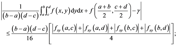
(3) If  is convex on the co-ordinates on
  and
and , then the following inequality holds:
 (6)
(6)
where

Remark 1. The Inequality (6) shows the result of giving the Inequality (5) an improved and simplified constant.
In [12] , Sarikaya et al. established the following results that gave an estimate of the difference in the right side of the Inequalities (3) for differentiable co-ordinated convex functions on .
.
Theorem 3. Let  be a partial differentiable mapping on
 .
.
(1) If  is convex on the co-ordinates on
 , then the following inequality holds:
 (7)
(7)
(2) If  is convex on the co-ordinates on
  and
and ,
,  , then the following inequality holds:
 (8)
(8)
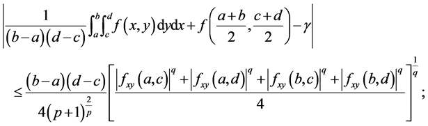
(3) If  is convex on the co-ordinates on
  and
and , then the following inequality holds:
 (9)
(9)
where

Remark 2. The Inequality (9) shows the result of giving the Inequality (8) an improved and simplified constant.
The goal of this paper is to establish an inequality which could be connected with the left side and right side of the extended Hadamard’s Inequality (3) and improve and generalize the Theorem 2 and Theorem 3. Also, the paper aims to note some consequent applications to special means.
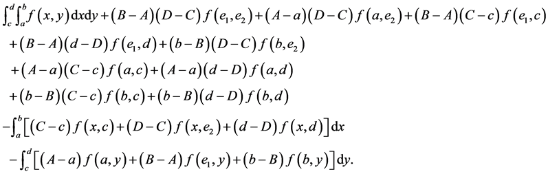
In order to show our main results, we need the following identities (I)-(VI):
(I) For ,
,  , the following four identities hold:


(II) For ,
,  , the following four identities hold:


(III) For ,
,  , the following four identities hold:


(IV) For ,
,  , the following four identities hold:


2. Main Results
In this section, let the mapping  for all
  be defined as follows:
 (10)
(10)
In order to prove our main results, we need the following lemma:
Lemma 1. Let  be a partial differentiable mapping on
 . Then the following inequality holds:
 (11)
(11)
where


Proof. It suffices to note that
 (12)
(12)
Integration by parts, we have


and

By summing the above four identities ,
,  ,
,  and
and  and simplifying the result, it follows that
 (13)
(13)
Then, multiply both sides by  in (12). From (12) and (13), we get the equations
  and
and . This proof of the identity 11 is complete.
Now, we are ready to state and prove the main results.
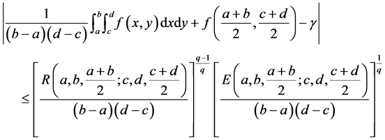
Theorem 1. Let  be defined as Lemma 1. If
  and the mapping
  is convex on the co-ordinates on
 then
then
 (14)
(14)
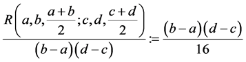
where

and
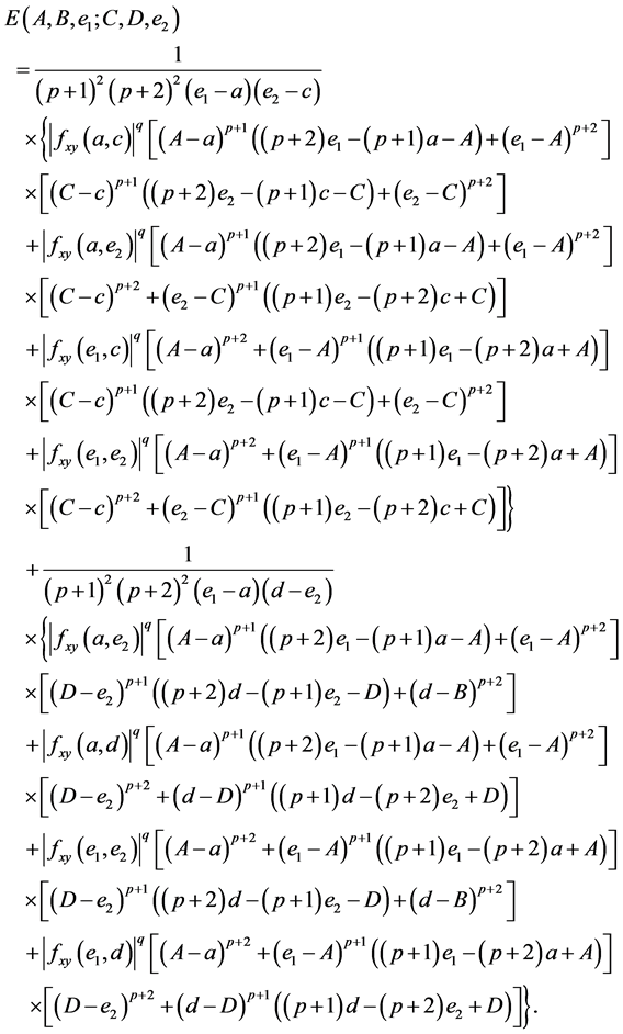

Proof. By using the identity (11), we have

If ,
,  , it follows from the power mean inequality that
 (15)
(15)
We denote  and
and  by
by

and

respectively, and then
 (16)
(16)
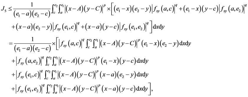
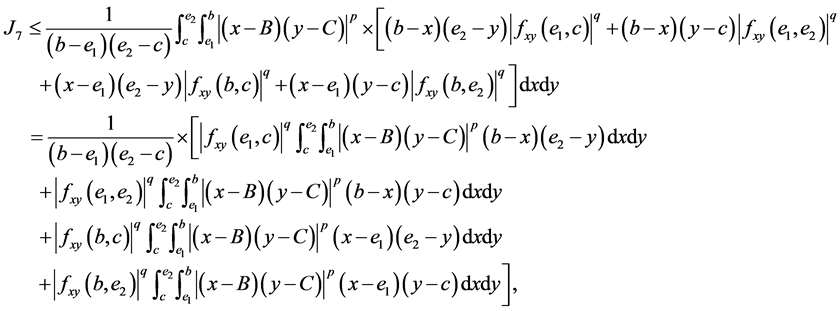
By using the integration techniques, we have

and similary we get,


and

By summing the above four identities ,
,  ,
,  and
and  and simplifying the result. Then according to (16), we get the estimated bound
 .
.
On the other hand, by using the identity mappings

and

we have
 (17)
(17)
By the convexit3 of  on the co-ordinates on
  and the Inequality (2) in
 ,
,  ,
,  and
and , then we have

and


By applying the identities (I), (II), (III) and (IV) to the above four inequalities and then simplifying the results, we get the estimated bound  and the Inequality (14) for
 . If
. If , then the Inequality (14) follows from (15) and (17). The proof of the Inequality (14) is complete.
Corollary 1. Under the assumptions of Theorem 1 with ,
,  ,
,  ,
,  ,
,  and
and , we have
 (18)
(18)
where  is as given in Theorem 2,

and

The Corollary 1 shows that we get the new estimated bound of the Inequality (6).
Corollary 2. Under the assumptions of Corollary 1 with , we have
 (19)
(19)
where  is as given in Theorem 2,
and


Remark 3. By using the convexity of  on the co-ordinates on
 , we have the inequality

and then

Hence the Inequality (19) improves the Inequality (6).
Remark 4. Under the assumptions of Theorem 1 with ,
,  ,
,  ,
,  ,
,  ,
,  and
and , we get the new estimated bound and it could improve the Inequality (4).
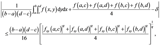
Corollary 3. Under the assumptions of Theorem 1 with ,
,  , we have
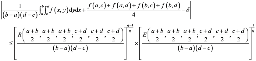 (20)
(20)
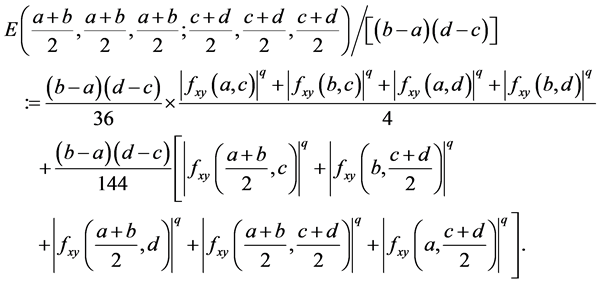
where  is as given in Theorem 3,

and


The Corollary 3 shows that we get the new estimated bound of the Inequality (9).
Corollary 4. Under the assumptions of Corollary 3 with , we have
 (21)
(21)
where  is as given in Theorem 3,

and
Remark 5. By using the convexity of  on the co-ordinates on
 , we have the inequality
and then

Hence the Inequality (21) improves the Inequality (9).
Remark 6. Under the assumptions of Theorem 1 with ,
,  and
and , we get the new estimated bound and it could improve the Inequality (7).
Example 1. Let the function  be
be ,
, . Then the result of the right-hand side of (6) or (9) is
 , whereas the right-hand side of (19) and (21) are
  and
and , respectively.
3. Some Applications to Special Means
As in [11] we shall consider extensions of arithmetic, logarithmic and generalized logarithmic means from positive real numbers. We take

where  is the set of integers.
Proposition 1. Let ,
,  ,
,  ,
,  ,
,  ,
,  ,
,  ,
,  , and
, and ,
,  ,
,  and
and . Then, for
 , we have
 (22)
(22)
Proof. The proof is immediate from Corollary 4 with ,
,  ,
,  ,
,  ,
, .
.
Proposition 2. Suppose ,
,  ,
,  ,
,  ,
,  ,
,  ,
,  ,
, . Then, for
 , we have
 (23)
(23)
Proof. The result follows from Corollary 4 with 

Remark 7. The Corollary 2 could also be applied to some special means.
Acknowledgements
The author is very grateful to the reviewers for carefully reading this paper and giving constructive comments.
NOTES
*2000 Mathematics Subject Classification. Primary 26D15. Secondary 26A51.