1. Introduction
Consider the following Hamilton-Jacobi-Bellman (HJB) equation:
 (1.1)
(1.1)
where  is a bounded domain in
  are elliptic operators of second order. Equation (1.1) is arising in stochastic control problems. See [2] and the references therein.
Equation (1.1) can be discretized by finite difference method or finite element method. See [1] [3] and the references therein. Then we obtain the following discrete HJB equation:
 (1.2)
(1.2)
where . Equation (1.2) is a system of nonsmooth nonlinear equations. Many numerical algorithms for solving (1.2) have been proposed. See [4] -[12] and the references therein.
[1] has given two iterative algorithms for solving (1.2). At each iteration, a linear complementarity subproblem or a linear equation system subproblem is solved. See also [4] .
Scheme I.
Step 1: Given  for some
  we find
  such that
Step 2: Let 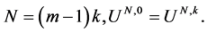 For
For  we find
  such that
Step 3: If 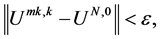 then the output is
  otherwise
  and it goes to Step 2.
Assume ![]() Let
Let
![]() (1.3)
(1.3)
That is: the lth row of matrix ![]() is the lth row of matrix
is the lth row of matrix![]() ; the lth component of vector
; the lth component of vector ![]() is the lth component of vector
is the lth component of vector![]() . Now we formulate Scheme II of Lions and Mercier in the notation above.
. Now we formulate Scheme II of Lions and Mercier in the notation above.
Scheme II.
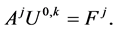
Step 1: ![]() for some
for some ![]() we find
we find ![]() such that
such that
![]() (1.4)
(1.4)
Step 2: For ![]() we find
we find ![]() such that
such that
![]() (1.5)
(1.5)
Step 3: Compute ![]() as the solution of
as the solution of
![]() (1.6)
(1.6)
Step 4: If ![]() then the output is
then the output is![]() , otherwise
, otherwise ![]() and it goes to Step 2.
and it goes to Step 2.
In the last decade many numerical schemes have been given for solving (1.2). But the above schemes are still playing a very important role. See [4] -[6] and the references therein.
In this paper we propose, based on Scheme II above, a relaxation scheme with a parameter![]() , which for
, which for ![]() is just Scheme II. In our numerical example, the new scheme with
is just Scheme II. In our numerical example, the new scheme with ![]() is faster than Scheme II
is faster than Scheme II![]() . The monotone convergence of the new scheme has been proved.
. The monotone convergence of the new scheme has been proved.
2. New Scheme and Convergence
We propose a new scheme which is an extension of Scheme II.
New Scheme II.
Step 1: Given ![]()
![]() for some
for some ![]() find
find ![]() such that
such that
![]() (2.1)
(2.1)
Step 2: For ![]() find
find ![]() such that
such that
![]() (2.2)
(2.2)
Step 3: Compute ![]() as the solution of
as the solution of
![]() (2.3)
(2.3)
Step 4: Compute
![]() (2.4)
(2.4)
Step 5: If ![]() then output
then output ![]() otherwise
otherwise ![]() and go to Step 2.
and go to Step 2.
In [13] we proposed the following conditions for (1.2).
Condition ![]() All the matrices
All the matrices ![]() are M-matrices.
are M-matrices.
In [13] we have proved the following theorem.
Theorem 2.1 If Condition ![]() holds then (1.2) has a unique solution.
holds then (1.2) has a unique solution.
We have the following convergence theorem.
Theorem 2.2 Assume that Condition ![]() holds, and that
holds, and that ![]() are produced by New Scheme II. Then
are produced by New Scheme II. Then ![]() is monotonely decreasing and convergent to the solution of (1.2).
is monotonely decreasing and convergent to the solution of (1.2).
Proof Since all ![]() are M-matrices,
are M-matrices, ![]() in New Scheme II are well defined.
in New Scheme II are well defined.
First, we prove ![]() is decreasing monotonically, i.e.,
is decreasing monotonically, i.e.,
![]() (2.5)
(2.5)
By (2.3) we have
![]() (2.6)
(2.6)
which combining with (2.1) and (2.2) yields
![]() (2.7)
(2.7)
Since ![]() are M-matrices, (2.7) means
are M-matrices, (2.7) means
![]() (2.8)
(2.8)
By (2.4) we obtain
![]() (2.9)
(2.9)
By![]() , (2.8) and (2.9) we know
, (2.8) and (2.9) we know
![]() (2.10)
(2.10)
and
![]() (2.11)
(2.11)
which and (2.10) implies
![]()
Similarly, by (2.3) we derive
![]()
which combining with (2.2) and (2.6) implies
![]()
Hence we have
![]() (2.12)
(2.12)
By (2.4), we have
![]() (2.13)
(2.13)
By (2.12), (2.13) and![]() , we know
, we know
![]() (2.14)
(2.14)
which combining with ![]() and (2.11) we derive
and (2.11) we derive
![]() (2.15)
(2.15)
By (2.11), (2.12) and (2.13) ,we get
![]()
which combining with (2.15) implies
![]()
It is easy to derive by induction that
![]() (2.16)
(2.16)
and
![]() (2.17)
(2.17)
It follows that (2.5) holds.
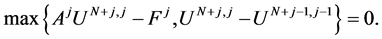
It follows from (2.2) and (2.3) that
![]() (2.18)
(2.18)
Since the set ![]() is a finite set there exist positive integers
is a finite set there exist positive integers ![]() and
and ![]() with
with ![]() such that
such that
![]()
Therefore, we have
![]()
![]()
Then by (2.2) we obtain
![]()
which and (2.17) results in
![]() (2.19)
(2.19)
From (2.4), (2.16) and (2.19) we have
![]() (2.20)
(2.20)
It follows from (2.18), (2.19) and (2.20) that
![]()
which means ![]() is a solution of (1.2). The existence of solution has been proved.
is a solution of (1.2). The existence of solution has been proved.
Finally, we prove the uniqueness of solution. Assume ![]() and
and ![]() are solutions of (1.2), i.e.,
are solutions of (1.2), i.e.,
![]() (2.21)
(2.21)
![]() (2.22)
(2.22)
It is easy to see from (2.21) and (2.22) that there exist ![]() and
and ![]() such that
such that
![]() (2.23)
(2.23)
![]() (2.24)
(2.24)
![]() (2.25)
(2.25)
![]() (2.26)
(2.26)
(2.23) and (2.26) implie![]() . But (2.24) and (2.25) implies
. But (2.24) and (2.25) implies![]() . Hence
. Hence![]() . The proof is complete. ,
. The proof is complete. ,
3. Numerical Example
We use example 2 in [4] , i.e., ![]()
![]() (3.1)
(3.1)
where ![]()
![]()
![]()
![]()
![]()
The discretization of the above second order derivatives are:
![]()
![]()
where ![]() denote the forward and backward difference respectively in
denote the forward and backward difference respectively in ![]() and
and![]() ,
, ![]() ,
,![]() . We use New Scheme II to solve the discrete problem. Take
. We use New Scheme II to solve the discrete problem. Take![]() ,
, ![]() and 1.1, 1.3, 1.5, 1.8, 1.9 respectively.
and 1.1, 1.3, 1.5, 1.8, 1.9 respectively.
Table 1 and Table 2 show the ∞-norm of the residual ![]() when iteration terminates.
when iteration terminates.
We see that ![]() for
for ![]() and
and ![]() is big for
is big for![]() .
.
Table 3 shows the relation between iteration number ![]() and relaxation number
and relaxation number![]() . Table 4 and Table 5 show the value of
. Table 4 and Table 5 show the value of ![]() at
at ![]() for
for ![]() and
and ![]() respectively.
respectively.
We can see from Table 3 that the algorithm for ![]() is faster than that for
is faster than that for![]() . Table 4 and Table 5 display the monotonicity of the algorithm.
. Table 4 and Table 5 display the monotonicity of the algorithm.
Funding
This work was supported by Educational Commission of Guangdong Province, China (No. 2012LYM-0066) and the National Social Science Foundation of China (No. 14CJL016).