On the Functional Empirical Process and Its Application to the Mutual Influence of the Theil-Like Inequality Measure and the Growth ()
1. Introduction
In many cases, one has to monitor a specific situation through some risk measure J on some population. The variation of J over time is called growth in case of negative variation and recession alternatively. This growth or recession is not itself sufficient to describe the improvement or deterioration of the situation. Often, the distribution of the underlying variable over the population should also be taken into account in order to check whether the growth concerns a great number of individuals or is rather concentrated on a few numbers of them.
In the particular case of welfare analysis, one may measure poverty (or richness) with the help of poverty indices J based on the income variable X. Over two periods s = 1 and t = 2, we say that we have a gain against poverty when , or simply a growth against poverty. Before claiming any victory, one must be sure that, meanwhile, the income did not become more unequally distributed, that is the appropriate inequality coefficient I did not increase. One can achieve this by studying the ratio
 .
.
To make the ideas more precise, let us suppose that we are monitoring the poverty scene on some population over the period time [1,2] and let  be the income variable of that population at periods 1 and 2. Let us consider one sample of
  individuals or households, and observe the income couple
 ,
, . For each period
 , we assume that Xi is strictly positive, and we compute the poverty measure
  and the inequality measure
 . We draw the attention of the reader that we consider here classes of measures both for poverty and inequality rather than specific ones. This leads to the very general results but requires extended notation.
For poverty, we consider the Generalized Poverty Index (GPI) introduced by Lo at al. [1] and Lo [2] as an attempt to gather a large class of poverty measures reviewed in Zheng [3] defined as follows for period i,
 (1)
(1)
where 
 is the income level representing the poverty line,
  is the number of poor,
  and
and  are constants,
  ,
,  , and
, and  are mesurable functions of

 and
and  By particularizing the functions A and w and by giving fixed values to the
  we may find almost all the available indices, as we will do it later on. In the sequel, (1) will be called a poverty index (indices in the plural) or simply a poverty measure according to the economists’ terminalogy.
This class includes the most popular indices such as those of Sen [4], Kakwani [5], Shorrocks [6], ClarkHemming-Ulph [7], Foster-Greer-Thorbecke [8], etc. See Lo [2] for a review of the GPI. From the works of many authors ([9,10] for instance),  is an asymptotically sufficient estimate of the exact poverty measure
 (2)
(2)
where  is the distribution function of
 , and L is some weight function.
As for the inequality measure, we use this Theil-like family, where we gathered the Generalized Entropy Measure, the Mean Logarithmic Deviation [11-13], the different inequality measures of Atkinson [14], Champernowne [15] and Kolm [16] in the following form:
 (3)
(3)
where  denotes the empirical mean while
 ,
,  ,
,  and
and  are measurable functions.
The inequality measures mentioned above are derived from (3) with the particular values of  and
and  as described below for all
 :
:
• Generalized Entropy
• 
• Theil’s measure:
• 
• Mean Logarithmic Deviation
• 
• Atkinson’s measure:
• 
• Champernowne’s measure:
• 
• Kolm’s measure:

We will see below that  converges to the exact inequality measure
 (4)
(4)
where  is the mathematical expectation of
  that we suppose to be finite here.
Each measure of the Theil-like family has its own particular properties, derived from the combination of different concepts. One may mention the concept of welfare criteria (Atkinson [14], Sen [17]), that of the analogy with analysis of risks (Harsanyi [18,19]; Rothschild and Stiglitz [20]), the complaints approach (Temkin [21]) etc. The Theil inequality itself finds all its interest in the information-theoretic idea following that of main components (Kullback [22]) and based on the three axioms (Zero-valuation of certainty, Diminishing-valuation of probability, Additivity of independent events). A deep review of such of individual properties for a number inequality measures can be found in Cowell [13,23,24] for instance.
It is worth mentioning that the TLIM presented here is rather a mathematical form gathering of a number of different measures having different insights. Its main interest is to provide a general and uniform approach for dealing with both poverty and inequality measures in the same time and to avoid details and repetitions, in a coherent framework for useful comparison studies. In coming papers, the families presented by Cowell [13,23,24] will be studied in similar ways.
The motivations stated above lead to the study of the behavior of

as an estimate of the unknown value of

Precisely confidence intervals of

will be an appropriate set of tools for the study of the influence of each measure on the other.
To achieve our goal we need a coherent asymptotic theory allowing the handling of longitudinal data as it is the case here and a stochastic process approach leading to asymptotic subresults with the help of the continuity mapping theorem.
We find that the functional empirical process, in the modern setting of weak convergence theory, provides that coherent asymptotic theory.
Indeed, we use bidimensional functional empirical processes  and its stochastic Gaussian limit
  to entirely describe the asymptotic behaviour of
  in the Gaussian field of
  and then find the law of
  as our best achievement.
The remainder of the paper is organized as follows. In Section 2, we remind key definitions and properties for functional empirical processes, and we state the asymptotic representation of the GPI of Sall and Lo [25] stated in Theorem 1 that will be used later on. In Section 3, we give our main results and make some commentaries and data driven applications to Senegalese pseudo-panel data are considered while the proofs and the tables are postponed in an appendix Section 5. Section 4 concludes.
2. Functional Empirical Process and Representation of GPI
2.1. A Brief Reminder on Functional Empirical Processes
Let  be a sequence of independent and identically distributed (i.i.d.) random elements defined on the probability space
  with values in some metric space
 . Given a collection
  of mesurable functions
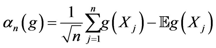
 , the functional empirical process (FEP) is defined by:

This process is widely studied in van der Vaart [26] for instance. It is directly seen that whenever
 , one has

and  where
where
 (5)
(5)
as consequences of the real Law of Large Numbers (LLN) and the real Central Limit Theorem (CLT).
When using the FEP, we may be interested in uniform LLN’s and weak limits of the FEP considered as stochastic processes. This gives the so important results on Glivenko-Cantelli classes and Donsker ones. Let us define them here (for more details see [26,27]).
Since we may deal with non measurable sequences of random elements, we generally use the outer almost sure convergence defined as follows. Remind that a sequence  converges outer almost surely to zero, denoted by
  whenever there is a measurable sequence of measurable random variables
  such that 1)
2) 
The weak convergence generally holds in  the space of all bounded real functions defined on
  equipped with the supremum norm

Definition 1 A class  is a GlivenkoCantelli class for
 , if
, if

Definition 2 A class  is a Donsker class for
 , or
, or  -Donsker class if
  converges in
  to a centered Gaussian process
  with covariance function

Remark 1 When  and
and ,
,  is the real empirical process and is denoted by
In this paper, we only use finite-dimensional forms of the FEP, that is  And then, any family
  of measurable functions satisfying (5), is a Glivenko-Cantelli and a Donsker class, and hence

where  is the Gaussian process, defined in Definition 2.
We will make use of the linearity property of both  and
and . Let
. Let  be measurable functions satisfying (5) and
 , then

The materials defined here, when used in a smart way, lead to a simple handling the problem tackled here.
2.2. Representation of the GPI
In this paper, we use the GPI in a unified approach that leads to an asymptotic representation for a large class of indices classified in three kinds.
First we consider the threshold condition:
(H1) There exist  and
and  such that,

Next we have form conditions (on the indices):
(H2a) There exist a function  where
where  and a function
  where
where  such that, when

(H2b) There exists a function  with
with  such that, when

Further we need regularity conditions on  and
and :
:
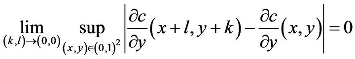
(H3) The functions  and
and  have uniformly continuous partial derivatives, that is
and

(H4) The functions  and
and  are monotonous.
(H5) The distribution function  is increasing.
(H6) There exist  and
and  such that
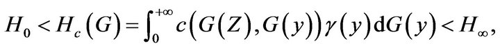
and

where  and
and  for
for .
.
Based on these hypotheses, we put


with


where


and

Now recall the functional empirical process
and introduce

the reduced process of Sall et Lo (see [25]).
The representation results of [25] for the GPI is the following.
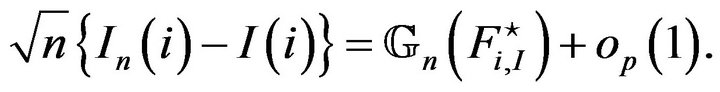
Theorem 1 Suppose that (H1)-(H6) are true, then we have the following representation
 (R)
(R)
Although these conditions may appear complicated, they are simple to check in usual cases with the popular poverty measures. We will see this in Section 3.
We are going to state our main results.
3. Results and Commentaries
3.1. Notations
Let us consider the following Renyi representations. Let
 and
and  two sequences of independent uniform rv’s on
 . Then we have the representation, meant as equalities in distribution:

where  is the generalized inverse of
 . We suppose that
  is continuous. The copula associated with the couple
  is defined by

where G1,2 is the joint distribution function of .
.
Next we consider the bidimensional functional empirical process based on , for some Donsker class
 :
:

and the limiting centered Gaussian stochastic process  its variance-covariance function defined by, for
 :
:

where

Now we introduce the following notations based on the functions ,
,  ,
,  ,
,  of (3) and on the functions
  and
and  of Theorem 1. The subscript
  refers to the period. The following series of notations are about the variation of the inequality measures and are listed below. Let us first denpte:

and next, for all ,
,

where  is the
  projection on

And finally,

with  and
and

where ,
,  and
and  are respectively the derivatives of the functions
 and
and 
For our results on the variation of the GPI, we need the functions  and
and  provided by the representation of Theorem 1. Put accordingly with these functions:

We define for all 

where  is the indicator function on the set

and

3.2. Main Theorems
We are now able to state our theorems. The first concerns the variation of the inequality measure.
Theorem 2 Let  finite for
  and let each
  continuously differentiable at each
 ,
, . Let
. Let 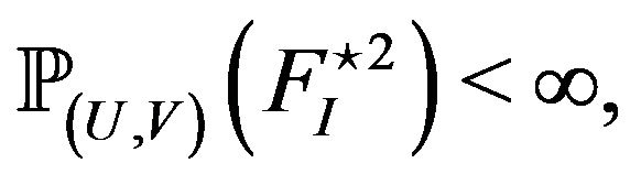 then we have the following convergence as

where  stands for the convergence in distribution and

The second concerns the variation of the GPI.
Theorem 3 Let  finite for
 . Suppose that

 and
and  are finite. Then

which is a centered Gaussian process of variance-covariance function:

where


with


and

Thus last one handles the ratio of the two variations.
Theorem 4 Supposing that the above mentioned hypotheses are true, then

with

and

In this case, let

then we have  tends to a functional Gaussian process

of covariance function

3.3. Commentaries
First of all, the results cover a large class of poverty measures and inequality indices. This explains why the notations seem heavy. Secondly, the variances of the limiting Gaussian processes seem also somehow tricky. But all of them are easily handled by modern computation means. We are going to particularise our results for famous measures and provide workable software codes for the computations.
3.4. Representation of Some Poverty Indices
We may easily find the functions g and  for the most common members of the GPI family (see [25,28]) in Table 1.
Where

and

with


And


where

and

Notice that the functions are indexed by  for the Kakwani measure. For the FGT measure of index
 , we have that
  and
and

3.5. Datadriven Applications and Variance Computations
3.5.1. Variance Computations for Senegalese Data
We apply our results to Senegalese data. We do not really have longitudinal data. So we have constructed pseudo-panel data of size , from two surveys: ESAM II conducted from 2001 to 2002 and EPS from 2005 to 2006. We get two series
  and
and . We present below the values of
  denoted here
 ,
,  denoted here
  and
and  denoted here
 .
.
When constructing pseudo-panel data, we get small sizes like n = 116. We use these sizes to compute the asymptotic variances in our results by mean of nonparametric methods. In real contexts, we should use high sizes comparable to those of the real databases, that is around ten thousands, like in the Senegalese case. Nevertheless, we back on medium sizes, for instance n = 696, which give very accurate confidence intervals.We use here the abreviations are given in Table 2.
The obtained confidence intervals are described in Tables 3 to 10, in Subsection 5.2. Before we present the outcomes, let us say some words on the packages. We provide different R script files at:
http://www.ufrsat.org/lerstad/resources/mergslo01.zip The user should already have his data in two files data1.txt and data2.txt. The first script file named after gamma_mergslo1.dat provides the values of ,
,  and
and  for the FGT measure for
  and for the six inequality measures used here. The second script file named as gamma_mergslo2.dat performs

Table 1. Specific functions of the poverty measures.

Table 3. Variations of the inequality indices.

Table 4. Variations of the poverty indices.

Table 5. Ratio of the variations with Shorrocks measure.

Table 6. Ratio of the variations with Sen measure.

Table 7. Ratio of the variations with Kakwani (2) measure.

Table 8. Ratio of the variations with FGT (1) measure.

Table 9. Ratio of the variations with FGT (0) measure.

Table 10. Ratio of the variations with FGT (2) measure.
the same for the Shorrocks measure. Lastly, gamma_ mergslo3.dat concerns the kakwani measures. Unless the user uploads new data1.txt and data2.txt files, the outcomes should be the same as those presented in the Appendix.
3.5.2. Analysis
First of all, we find in Tables 3 and 4 in the appendix 5 that at an asymptotical level, all our inequality measures and poverty indices used here have decreased. When inspecting the asymptotic variance, we see in Table 4 that for the poverty indice, the FGT and the Kakwani classes respectively for ,
,  and k = 1, k = 2 have the minimum variance, specially for
  and k = 2. This advocates for the use of the Kakwani and the FGT measures for poverty reduction evaluation. As for the inequality approach in Table 3, it seems that Atkinson measure ATK (0.5) has the minimum variance and then is recommended.
As for the ratio of the poverty index over the inequality
measure, we have a dependence of over 50% for the following couples in Table 11, that we can find in Tables 5 to 8.
The maximum ratio 3.024 is attained for FGT (0) and Atkinson (0.5). Based on these data, and on the confidence intervals in Table 9, we would report at least of 46.43% for these two measures and conclude that the gain over poverty in Senegal between these two periods is significally pro-poor. We would have worked with all couples with a ratio over 50% to have the same conclusion.
The present analysis should be developped in a separated paper research since this one was devoted to a theoritical basis. We plan to apply at a regional basis, that is for the countries of the UEMOA in West Africa.
4. Conclusion
We have been able to compute confidence intervals for the ratio of variations for the poverty and the inequality indices. The results enabled us to cheek whether the growth is pro or against poor in Senegal from 2002 to 2006. It always remains to undertake large scale data driven applications at a regional level, precisely in the UEMOA African area. We used in this paper a Theil-like family of inequality measures that does not include the celebrated and important Gini index. Moreover other the Theil-like families exist. It would be interesting to have the same theory developed here using the Gini index and other families as well. We plan to do it in a very close future.
5. Acknowledgements
We express our thanks to the Ministère de l’Enseignement Supérieur et de la Recherche for financial support under a FIRST grant 2013-2014.
Appendix
Proofs of the Theorems
Proof of Theorem 2.
By using the delta-method, we have for all :
:

Then
 (6)
(6)
Similarly, we have
 (7)
(7)
From this and (3.1), we have

and then
 (8)
(8)
Further

But

Thus

that is
 (9)
(9)
Finally using the linearity of the FEP, we get

and conclude by
 (10)
(10)
and

Proof of Theorem 3. We have

and then

We arrive at
 (11)
(11)
We get the variation of  between to instants
  and
and  as follows

This leads to

The proof will be complete with the expression of . We have

Let us compute these three numbers. First consider,

Secondly, compute

By developing and applying Fubini to this term, we get

or


then

and

Similarly we obtain


But

By identification, we get

and remind that these quantities were defined in Theorem (3). Finally, we have

This achieves the proof of Theorem (3).
Proof of Theorem 4.
By (6) and (10), is clear that

is asymptotically Gaussian with covariance

Then

Next straightforward computations yield

Then

We finish by computing its variance . For this, let

and

By using the notation of Theorem 4, where we introduced  and
and , we arrive at

This completely achieves the proofs.