1. Introduction
Fractional calculus is a classical mathematical concept, with a history as long as calculus itself. It is a generalization of ordinary differentiation and integration to arbitrary order, and is the fundamental theories of fractional order dynamical systems. Fractional-order differential/integral has been applied in physics and engineering, such as viscoelastic system [1], dielectric polarization [2], electrode-electrolyte polarization [3] and electromagnetic wave [4], and so on.
The fractional order system and its potential application in engineering field become promising and attractive due to the development of the fractional order calculus. Typically, chaotic systems remain chaotic when their equations become fractional. For example, it has been shown that the fractional order Chua’s circuit with an appropriate cubic nonlinearity and with an order as low as 2.7 can produce a chaotic attractor [5].
However, there are essential differences between ordinary differential equation systems and fractional order differential systems. Most properties and conclusions of ordinary differential equation systems cannot be extended to that of the fractional order differential systems. Therefore, the fractional order systems have been paid more attention. Recently, many investigations were devoted to the chaotic dynamics and chaotic control of fractional order systems [6-12].
In this paper, practical scheme is proposed to eliminate the chaotic behaviors in fractional order system by extending the nonlinear feedback control in ODE systems to fractional-order systems. This paper is organized as follows. In Section 2, the numerical algorithm for the fractional order system is briefly introduced. In Section 3, Dynamics of the fractional order system is numerically studied. In section 4, general approach to feedback control scheme is given, and then we have extended this control scheme to fractional order system, numerical results are shown. Finally, in Section 5, concluding comments are given.
2. Fractional Derivative and Numerical Algorithm
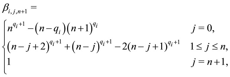
There are two approximation methods for solving fractional differential equations. The first one is an improved version of the Adams-Bashforth-Moulton algorithm, and the rest one is the frequency domain approximation. The Caputo derivative definition involves a time-domain computation in which nonhomogenous initial conditions are needed, and those values are readily determined. In this paper, the Caputo fractional derivative defined in [13] is often described by

when  is the first integer that is not less than
 ,
,  is the α-order Riemann-Liouville integral operator which defined by

where  is the Gamma function,
Now we consider the fractional order system [14] which is given by
 (1)
(1)
where  is the fractional order,
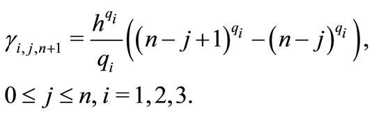
By exploiting the Adams-Bashforth-Moulton scheme [15], the fractional order system (1) can be discretized as followings:


3. Dynamic Analysis of the Fractional Order System
Theorem 1: The fractional linear autonomous system

is locally asymptotically stable if and only if

Theorem 2: Suppose  be an equilibrium point of a fractional nonlinear system

If the eigenvalues of the Jacobian matrix  satisfy
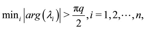
then the system is locally asymptotically stable at the equilibrium point 
The system (1) has five equilibrium points:

where 
When  we obtain

First, we choose 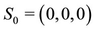 to study, the eigenvalues of the Jacobian matrix are
  and
and  We can obtain
  and
and  According to Theorem 2, we can easily conclude that the equilibrium
  of system (1) is unstable when
  and
and  are all greater than zero.
We choose  and
and  to study, the eigenvalues of the Jacobian matrix are
  and
and  We can obtain
  and
and  According to Theorem 2, we can easily conclude that when
  and
and  are all less than
  the equilibrium
  of system (1) is stable. On the contrary, when
  and
and  are all great than
 , the equilibrium
  of system (1) is unstable.
Finally , when choose 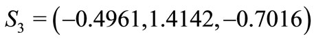 and
and 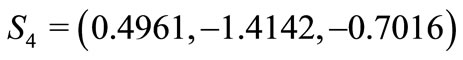 to study, the eigenvalues of the Jacobian matrix are
  and
and  We can obtain
 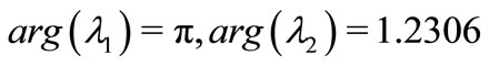 and
and  According to Theorem 2, we can easily conclude that when
  and
and  are all great than
 , the equilibrium
  of system (1) is unstable.
In sum, there exists at least one stable equilibrium  and
and  of system (1), when
  and
and  are all less than
 , i.e., the system (1) will be stabilized at one point
  finally; when
  and
and  are all greater than
 , all the equilibriums of system (1) are unstable, the system (1) will exhibit a chaotic behaviour; when
  the problem will be complicated, the system (1) may be convergent, periodic or chaotic. For example, when
  the value of the largest Lyapunov exponent is 0.1653. Obviously, the fractional order system (1) is chaotic. When
  the fractional order system (1) is not chaotic, but periodic orbits appear.
4. Feedback Control
Let us consider the fractional order system
 (2)
(2)
where  is the system state vector, and
  the control input vector. Given a reference signal
  the problem is to design a controller in the state feedback form:

where  is the vector-valued function, so that the controlled system

can be driven by the feedback control g(x, t) to achieve the goal of target tracking so we must have

Let  be a periodic orbit or fixed point of the given system (2) with
 , then we obtain the system error

where  and
and 
Theorem 3: If  is a fixed point of the system (2) and the eigenvalues of the Jacobian matrix at the equilibrium point
  satisfies the condition

then the trajectory  of system (2) converge to
Let us consider the fractional order system (2), we propose to stabilize unstable periodic orbit or fixed point, the controlled system is as follows:
 (3)
(3)
Since  is solution of system (1), then we have:
 (4)
(4)
Subtracting (4) from (3) with notation, 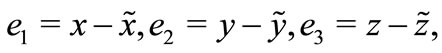 we obtain the system error
 (5)
(5)
We define the control function as follow
 (6)
(6)
So the system error (5) becomes
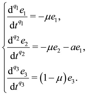 (7)
(7)
The Jacobian matrix of system (7) is

so we have the eigenvalues 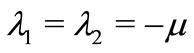 and
and  When
When  all eigenvalues are real negatives, one has
  therefore
  for all
  satisfies
  it follows from Theorem 3 that the trajectory
  of system (2) converges to
  and the control is completed.
5. Numerical Simulation
In this section we give numerical results which prove the performance of the proposed scheme. As mentioned in Section 2 we have implemented the improved AdamsBashforth-Moulton algorithm for numerical simulation.
The control can be started at any time according to our needs, so we choose to activate the control when  in order to make a comparison between the behavior before activation of control and after it.
For  and q3 = 0.98, unstable point
  has been stabilized, as shown in Figure 1, note that
 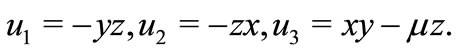 The control is activated when
  and the evolution of
  is chaotic, then when the control is started at
  we see that
  is rapidly stabilized.
For  and
and 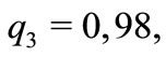 the unstable point
  has been stabilized, as shown in Figure 2.
For 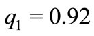 and
and  the unstable point
  has been stabilized, as shown in Figure 3.
For  the unstable point
  has been stabilized, as shown in Figure 4.
For  the unstable point
  has been stabilized, as shown in Figure 5.
When  is less than
 , there is a chaotic behavior,
Figure 1. Stabilizing the equilibrium point S0 for q1 = 0.93, q2 = 0.95 and q3 = 0.98.

Figure 2. Stabilizing the equilibrium point S1 for q1 = 0.93, q2 = 0.95 and q3 = 0.98.

Figure 3. Stabilizing the equilibrium point S2 for q1 = 0.92 and q2 = q3 = 0.97.

Figure 4. Stabilizing the equilibrium point S3 for q1 = q2 = q3 = 0.94.
Figure 5. Stabilizing the equilibrium point S4 for q1 = q2 = q3 = 0.96.
but when the control is activated at , the five points
  and
and  are rapidly stabilized.
6. Conclusions
Chaotic phenomenon makes prediction impossible in the real world; then the deletion of this phenomenon from fractional order system is very useful, the main contribution of this paper is to this end.
In this paper, we investigate the system with fractional order applying the fractional calculus technique. According to the stability theory of the fractional order system, dynamical behaviors of the fractional order system are analyzed, both theoretically and numerically. Furthermore, nonlinear feedback control scheme has been extended to control fractional order system. The results are proved analytically by stability condition for fractional order system. Numerically the unstable fixed points have been successively stabilized for different values of  and
and  Numerical results have verified the effectiveness of the proposed scheme.
7. Acknowledgements
This work is supported by the Qing Lan Project of Jiangsu Province under the Grant Nos. 2010 and the 333 Project of Jiangsu Province under the Grant Nos. 2011.
NOTES