Analysis of Winds Affecting Air Pollutant Transport atLa Plata, Argentina ()
1. Introduction
Urban areas are major sources of air pollution which is the result of processes of accumulation, dispersion, transformation and removal of contaminants. Pollutant emissions affecting air quality in cities have an adverse impact on human health [1]. The city of La Plata and its surroundings are densely populated areas (approximately 800,000 inhabitants) with high industrial and vehicular activity. Glassmann and Mazzeo [2] made a regional study of air pollution potential in Argentina and concluded that La Plata is located in a zone with poor atmospheric self-cleansing capacity. In spite of these facts, no governmental air monitoring network is installed. In recent years several works contributed to assess different parameters characterizing air pollutants in the area [3-7] but references to hourly distribution of winds and sealand breeze effects have been rare. The characterization of wind direction frequency patterns associated with industrial sources is essential for describing the transporttation of air pollutants and settles the basis for a further assessing of environmental impact on human health.
Enriching previous reports this article make available a detailed summary of wind direction frequencies while discusses their importance for air pollutant modeling.
One purpose of this paper is to compare observed wind direction frequency patterns covering the period 1998- 2003 at two monitoring sites (named Point A and J Figure 1). A previous report [8] analyzed similarity between both sites employing cluster and multidimensional scaling analysis. The present study is intended to gain insight of hourly occurrences of winds regarding air pollutants. To this end two different approaches are involved: one quantifies proximity using the squared Euclidean distance and the other quantifies correlation applying to the minimum covariance determinant (MCD) estimator. The well known squared Euclidean distance between two patterns expresses how far these two objects are from each other. It is in fact a dissimilarity measure [9] because the distance increases as the similarity decreases. Although non conventionally used in atmospheric sciences, the MCD coefficient (a linear robust correlation estimator) was adopted instead of the traditional Pearson’s coefficient because it reduces the influence of outliers [10]. Both similarity approaches are intended to reveal different aspects of wind pattern characteristics. While MCD allows comparing pattern “shapes”, Euclidean distance allows comparing “sizes” [11]. One wind pattern will be considered similar to another insofar as they are positively correlated and close one to each other.
In a previous work [12] two sectors relevant for the
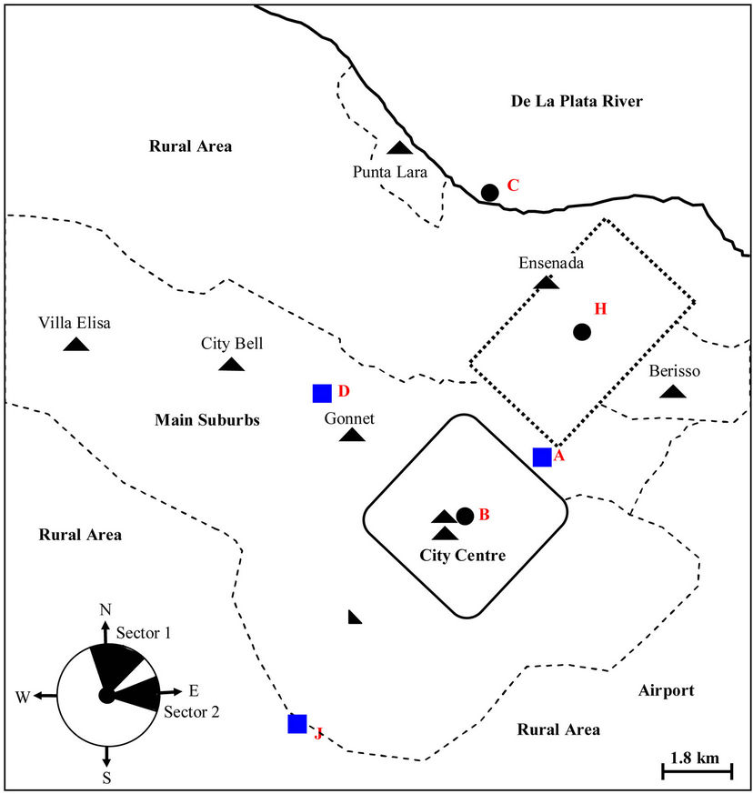
Figure 1. Map covering parts of La Plata and surroundings. Measurement points are indicated with a square and other reference points with a circle. Point A: National University of Technology. Point B: city center. Point C: river bank. Point D: Center of Optical Research (CIOp). Point H: center of the rectangle close to oil refinery plants. The rectangle (dotted lines) indicates the area with high industrial activity including a shipyard and steel plants. Point J: Agrometeorology Station. Sectors 1 and 2 are shown at the low left corner of the figure. Density of population is expressed qualitatively as two, one or half triangles depending on its degree. Dashed lines embrace main populated areas.
transport of air pollutants from the Industrial Pole to populated areas covering the period 1997-2000 have been emphasized, namely: Sector 1 (NNW-N-NNE-NE) transporting pollutants towards the city center and Sector 2 (ENE-E-ESE) transporting pollutants to main residential areas (see down left corner in Figure 1). In the present work the period under study is expanded and the discussion is intensified. The second purpose of this paper is to assess the presence of these sectors and to consider their daily and seasonal variations associated with the daily and annual cycles. Also their stability with time is evaluated by employing a local weighted non-parametric regression method (LOESS) increasingly used in environmental sciences [13,14]. The period involved to analyze both sectors is 1998-2003 for sites A and J (selected because of the availability of simultaneous data) and 1998- 2009 for site J (the largest data set available).
SO2 is often taken as a witness gas of industrial activity. An increasing annual trend was detected close to the Industrial Pole between 1998 and 2000, surpassing 26 ppbv for the year 2000 [15]. Being industrial air pollutant hourly data scarce, we employed observed SO2 concentrations published in a previous report for correlation purposes.
Additionally, observed seasonal averaged wind velocityies at both sites are compared taking into account differences in instrument exposure. Observed calms are provided for context.
2. Materials and Methods
2.1. Characteristics of the Region under Study
La Plata is located in eastern Argentina (35˚S, 58˚W) on the estuary of the De La Plata River, which is one of the most important rivers in South America (its basins covers 3,200,000 km2) and is part of the boundary between Argentina and Uruguay. The city centre is located about 11 km far from the Río de La Plata bank in the typical “Pampa” prairies (see Figure 1). The average elevation is 15 m above the mean sea level. La Plata River estuary is wide enough to have relevant sea-land circulations. From a geographical point of view the diurnal cycle of the sea-breeze is expected to occur between NNW and ESE (clockwise). According to Thornthwaite’s [16] classification La Plata climate is “wet, mesothermal with null or small water deficiency”. The annual mean temperature is 16˚C. January is the hottest month with 22.4˚C and July the coldest month with 9.9˚C. The annual average relative humidity is 70% with a minimum in January (60%) and a maximum in July (85%) [17]. According to the National Meteorological Service for the last three decades (1981-2010) predominant wind directions for 8-direction wind roses registered at La Plata Airport (see Figure 1) are E, NE and N [18-20].
A large Industrial Pole (including oil refinery plants, a major shipyard, steel processing plants, etc.) located between the river and the city (see Figure 1) concentrates major industrial air pollutants sources for the city and surroundings. A new thermal power station (with a capacity of 560 MW) constructed in the vicinity areas of the industrial complex is announced to be put in operation during 2012.
2.2. Instrumentation and Data Characteristics
Monitoring site labeled as Point A is located in a urban area and belongs to Universidad Tecnológica Nacional (UTN). It operates a Weather Monitor II Euro Version® meteorological station (Davis Instruments, CA). Monitoring site Point J is in a semi-rural area belonging to Estación Agrometeorológica Julio Hirschhorn-Universidad Nacional de La Plata (UNLP). It operates a GroWeather Industry® meteorological station (Davis Instruments CA). Both models take wind directions every 22.5˚ completing 360˚ of the compass (16 directions) with an accuracy of ±7˚ of the read out. The detection limit and resolution for wind velocities are 1.6 km·h–1 in both cases. The heights above the ground for the anemometers and weather cock were 12 m at Point A and 5 m at Point J. The distance from Point C (at the river bank see Figure 1) to Point A is around 9.8 km while to Point J is around 18 km.
Sets of simultaneous data at points A and J correspond to 1998-2003. Data at Point J covering the period 2004- 2009 were also employed. The data set belonging to site A had a deficiency in NNE records. This drawback was found to be due to an obstacle that prevented a correct observation. Both monitoring sites provided complete data sets with the exception of Point J during winter 2000 which records were very poor; missing data were replaced by the median of the 4 adjacent years (the choice of this number of years was arrived at as a consequence between bias and variance); the same procedure applied to summer, autumn and spring yielded the smallest quadratic error compared with the average and the weighted average. Data at Point A were recorded every 15 minutes while data at Point J were recorded every hour. The difference in data quality is due to the fact that the institutions from which the data were obtained use them for different purposes; these sets do not conform a monitoring network. Throughout this paper hourly averages imply hourly blocks (for example, 00:00-00:59 hr is equivalent to “hour 0” local time). Regarding seasons, summer included December of the precedent year and January and February of the current year, whereas autumn included March, April and May, winter included June, July and August and spring included September, October and November.
2.3. Similarity Analysis
Seasonal hourly patterns of wind direction frequencies for both monitoring sites were compared by considering DE2 (squared Euclidean Distance) and MCD (minimum covariance determinant).
The squared Euclidean distance is a metric that allows assessing proximity between two objects (vectors).
 (1)
(1)
where x and y are in our case objects of dimension 24.
Recall that Pearson product-moment sample correlation coefficient “r” can be expressed as:
 (2)
(2)
where

is the estimated covariance between variables x and y,  and
and  are the estimated variances of x and y, and
  and
and  are the estimates of their respective means. This statistic is widely used for summarizing the relationship between two variables or group of variables that define an object. The statistic r expresses the degree of association of two variables [21] and constitutes a standardized measure of linear dependence between them [22]. A value of r close to 1 or –1, indicates that each of the variables can be accurately predicted by a linear function of the other. The sign indicates the direction of the relationship between the Y and the X.
Two drawbacks have been traditionally accounted for the application of r [23,24]: the sensitivity of this statistic to outliers due to the fact that classical average and covariance matrices are extremely sensitive to atypical observations [25] and the inability to recognize nonlinear relationships. Outliers may play the role of inflating or deflating the r estimate since there are “good” and “bad” leverage points [25].
In order to minimize the influence of outliers we employed the MCD correlation coefficient introduced by Rousseeuw [10,26,27] that considers robust alternatives for the location and scatter estimates given in Equation (2).
MCD computes average and scatter estimates regarding a subset of h of the n data (2 < h < n) which attain the smallest determinant of the covariance matrix. Then, the location and scatter MCD estimators are given by the average and covariance matrix of the optimal subset. MCD will provide an estimate of the strength of the correlations for the data of interest free of the influence of outliers, so that a low value of the estimate would indicate that the linear relationship between the objects involved is poor. The fast-algorithm for computing MCD is complex and it is explained in detail in [28]. MCD computations have been carried out by the use of the statisticcal software package SCOUT Version 1.0 from US EPA [29]. MCD properties such as breakdown value, affine equivariance and influence function are described in [30, 31] and [32]. In order to have a wide coverage and supposed a 10% of contamination in our data, a value of h = 0.8 was chosen. Thereby the breakdown point (BDP) was about 20%, which is a value close to that recommended by [33] in order to have a balance between robustness and efficiency [25].
Distances and correlation coefficients are different approaches to measure similarity [34]. Two objects can be highly correlated (MCD ≈ 1 or –1), but their distance could be high enough to consider them as different (e.g. they could have a significantly different mean). On the other hand, the two objects can be poorly correlated (MCD ≈ 0) but DE2 could be very small and so they can both be considered as describing the same characteristics (although their differences may be due to different causes). Furthermore, according to [9] DE2 is very sensitive to additive and proportional translations while MCD is wholly insensitive to them; finally, both estimates share sensitiveness to mirror images translations. Then, for the purpose of comparing wind frequency patterns measured at two monitoring sites both correlation and proximity were considered of interest”
2.4. Assessing the Influence of the Day and the Season on Sectors 1 and 2
Wind frequencies for Sectors 1 and 2 at points A and J are considered. In order to discriminate and quantify “daily” from “seasonal” variations within the series, an “average day” was estimated by averaging hourly the corresponding hours of the day for all the data. The averaged day was later substracted to each original series. The remaining curve had still the influence of the season. The seasons through the years under study were then averaged to obtain the “average season”. The average season was later on substracted to the remaining curve (the curve resulting after the first subtraction) in order to obtain the residuals. Finally, the variances involved at the different steps of subtractions were considered in order to evaluate the degree of contribution of the “day” and the “season” to the total variation.
A trend analysis for Sectors 1 and 2 was performed as a prospective study in order to save the inexistence of simultaneous larger hourly data collections published in the area.
In both cases a nonparametric method based on local weighted regression, usually called “LOESS” or “LOW ESS” [35,36] was employed. For a sequence  the procedure computes at each given x within the range of the
 ’s a value
  as follows. Call I a window with span h around x: I = [x – h, x + h]. For
  compute weights
  where W is the “tricube” function
  for
for  and
and  otherwise. This function is maximal at x = 0 and decreases to zero at x = 1. Then for
  with
with  fit a quadratic polynomial by weighted least squares; that is, find
  such that

Finally put . It is usual to compute the fit at each observation, obtaining
 , but the fit can be performed at any point within the range of the
 ’s. The procedure is “nonparametric” in that the overall fitted curve
  has no explicit form and does not belong to any given parametric family. A small window span h yields a small bias but a possibly large variance, while the contrary happens with a large h; therefore h must be chosen to strike a balance between bias and variability. The nonparametric fit allows visualizing trends but it is important to discriminate whether it reveals actual data features or simply statistical artifacts. To this end the means corresponding to different time intervals were compared by estimating their standard deviations. Here it must be taken into account the lack of independence in the data. If
  is a stationary sequence with variance
  and
and  then [37]
  is to be computed, where V is the “inflation factor” [23]:
 ;
;  is the k-th order autocorrelation. An analysis of the data suggested that their dependence could be well represented by a first-order autoregressive process, with
  and therefore
Finally, the deviates for the mean were estimated for each window as the square root of the variance for the mean.
2.5. Exposure Corrections for Wind Velocities
An empirical approach often used in air pollutant dispersion calculations is the power law velocity profile [38,39] given by:
 (3)
(3)
where:
 is the wind velocity “corrected” to the height z according to terrain roughness and atmospheric stability given by p;
 is the wind velocity observed at a given height;
z is the height that is desired to obtain the “corrected” wind velocity;
 is the height for the observed wind velocity.
The exponent p increases with increasing surface roughness and increasing stability. Various researches reported p values between 0.07 and 0.60. Tables given in chapter 3 of [40] were used in order to select the most appropriate value for p at points A and J. In order to avoid differences due to the effect of altitude wind velocities were corrected considering a reference height of 10 m. Besides, differences in roughness (see Section 2.2) between points A and J, were saved by affecting each point with correction factors of p = 0.25 and p = 0.15 respectively. A neutral atmospheric stability class was considered due to the fact that the seasonal averages involve day and night.
3. Results and Discussion
3.1. Sea-Land Breeze Presence
Observed wind frequencies covering the 16 directions of the compass at sites A and J for the four seasons are analyzed on hourly basis. Figure 2 shows only summer and winter patterns due to space constraints; autumn and spring displayed in most cases intermediate behaviors. Considering the lack of meteorological studies in the area the sea-land breeze phenomenon appears as the only significant source of local atmospheric variability. Its influence is more pronounced during summer due to the higher temperature contrast between the land and the large water surface of the La Plata River. For this reason summer is considered the leading season to carry out the analysis.
An overview of Figure 2 shows that wind frequencies for E (e.g. Figure 2(a1)), N (e.g. Figure 2(a13)) and NE (e.g. Figure 2(a15)) are high respect to the rest of the directions throughout the seasons in coincidence with observations carried out at La Plata Airport (Section 2.1). According to Barros et al. [41] these three wind directions, originated by the western flank of the subtropical anticyclone of the South Atlantic Ocean (located around 35˚S, 45˚W), are of major importance for the De La Plata River basin.
During the night between hours 0 and 8 the frequencies for S (Figure 2(a5)) and SSW (Figure 2(a6)) are significantly higher than those of the rest of the day. This is attributable to land-breeze because these wind directions are somewhat perpendicular to the coastline. During the first morning hours these frequencies decrease notably. As far as the influence of southern winds diminishes, wind frequencies from N (Figure 2(a13)), NNE (Figure 2(a14)) and NE (Figure 2(a15)) start to gain importance during the morning (recall that low values for NNE at Point A are due to measurement deficiencies Section 2.2). These three directions are involved with the
first stage of the sea-breeze development that occurs during the morning hours when winds from the river start to blow towards the land. Winds flow then increasing the northerly component [42]. Sea-breeze winds follow a rotational pattern [43] clockwise, previously detected by Borque et al. [44] in a preliminary study during one day of March that revealed that the circulation rotates from NE to E between noon and dusk. This effect is observed in a second stage when N and NE winds decrease from hour 16 on (Figure 2(a13) and Figure 2(a14)) while ENE (Figure 2(a16)), E (Figure 2(a1)) and ESE (Figure 2(a2)) becomes dominant until they reach a peak during the evening (around hours 20 and 21).
Differences between points A and J for wind direction frequencies involving the land-breeze are smaller than those involving sea-breeze. A weaker land-breeze is expected mainly due to the nocturnal stability [42] but also to the city roughness that inhibits the flow of air from land to water. The wind direction spectrum observed for the land-breeze appears restricted respect to that for seabreeze. The inland penetration should be encouraged in future studies.
3.2. Similarity Analysis for Wind Direction Frequencies during the Period 1998-2003
The four seasons of the year show by inspection proximate patterns when comparing both sites (Figure 2). Warm seasons showed in general more differences between patterns than cold ones, as can be seen for summer and winter in Figure 2. This is attributable to the sealand breeze cycle that is more intense in warmer than in colder seasons [8].
Figure 2 shows major differences for NNE, NE and SE in summer while for NNE, NNW and N in winter. To analyze proximities between patterns in a more objective way the squared Euclidean distance (DE2) is employed (Table 1). This metric gives an overall estimate of the proximity between patterns but does not distinguish if the differences are concentrated in a few hours or distributed throughout the day. Therefore maximum individual differences between patterns (corresponding to one particular hour of the day) are also discussed in order to show a more complete picture of the proximity approach.
NE and NNE exhibit relative high distances throughout the seasons, often between oneand two-fold standard deviation from the mean (of DE2) (Table 1). Recalling that NNE has been deficiently measured at site A and that wind direction frequencies were expressed as a percentage for a given hour, it is possible to consider that the distortion for this direction would mainly affect the adjacent ones i.e. NE and N. Regarding these three directions the maximum individual differences throughout the day were: 12.9% in summer for NE at hour 13 (Figure 2 (a5)), 8.3% in autumn for NE at hour 12, 9.0% in winter for NNE at hour 16 (Figure 2(b14)) and 10.4 % in spring for NE at hour 11. Excluding these three directions, overall

Table 1. Squared Euclidean distances covering all the directions of the compass and the four seasons.
major differences involve SE and E in summer, SE and NNW in autumn, NNW and ENE in winter and SE and SW in spring (Table 1). Except for NNE, NE and N major individual differences are 13.4% for E in summer at hour 19 (Figure 2(a1)), 10.3% in autumn for E at hour 18, 8.7% in winter for NNW at hour 17 (Figure 2(b12)), 16.4% ESE in spring at hour 20. Recalling that the group of wind directions affected by sea-breeze circulation involves NNW-ESE clockwise, most of the differences found can be attributed to this mechanism. According to Oke [45] a wind parallel with the coastline, i.e. SE, is expected to be found when the inflow of the water surface decays, but at Point A this phenomenon is not remarkably evidenced, note that during the evening SE is more important at Point J than at Point A what suggests that a more complex pattern is occurring.
Directions comprehended between SSE and NW (clockwise) are in general proximate for all the seasons (all values are below the general mean) (Table 1). This group of directions involves cold fronts, frontal waves and instability lines. Considering that the area under analysis is mainly flat, the land-breeze is weak and that the directions involved are not influenced by sea-breeze phenomenon both weather stations show proximate patterns regarding wind occurrences.
Table 2 shows the MCD estimates for the same patterns discussed above. An overview of this table shows that linear relationship between patterns are somewhat alternated