Deriving CDF of Kolmogorov-Smirnov Test Statistic

Jan Vrbik

Department of Mathematics and Statistics, Brock University, St. Catharines, Ontario, Canada.

DOI: 10.4236/am.2020.113018                

Abstract

In this review article, we revisit derivation of the cumulative density function (CDF) of the test statistic of the one-sample Kolmogorov-Smirnov test. Even though several such proofs already exist, they often leave out essential details necessary for proper understanding of the individual steps. Our goal is filling in these gaps, to make our presentation accessible to advanced undergraduates. We also propose a simple formula capable of approximating the exact distribution to a sufficient accuracy for any practical sample size.

Keywords

Kolmogorov-Smirnov Test, Asymptotic Distributions, Generating Functions, Jacobi Theta

1. Introduction

The article’s goal is to present a comprehensive summary of deriving the distribution of the usual Kolmogorov-Smirnov test statistic, both in its exact and approximate form. We concentrate on practical aspects of this exercise, meaning that

• reaching a modest (three significant digit) accuracy is usually considered quite adequate,

• computing critical and P-values of the test is the primary objective, implying that it is the upper tail of the distribution which is most important,

• methods capable of producing practically instantaneous results are preferable to those taking several seconds, minutes, or more,

• simple, easy to understand (and to code) techniques have a great conceptual advantage over complex, black-box type algorithms.

This is the reason why our review excludes some existing results (however deep and mathematically interesting they may be); we concentrate only on the most relevant techniques (this is also the reason why our bibliography is deliberately far from complete).

1.1. Test Statistic

The Kolmogorov-Smirnov one-sample test works like this: the null hypothesis states that a random independent sample of size n has been drawn from a specific (including the value of each of its parameters, if any) continuous distribution. The test statistics (denoted $D_n$ ) is the largest (in the limit-superior sense) absolute-value difference between the corresponding empirical cumulative density function (CDF) and the theoretical CDF, denoted $F\left(x\right)$, of the hypothesized distribution; the former is defined by

(1)

where $X_1\mathrm{,}{X}_2,\cdots ,X_n$ are the individual sample values and $I_{X_i<x}$ is the usual indicator function (equal to 1 when $X_i$ is smaller than x, equal to 0 otherwise). Note that $F_e\left(x\right)$ is a step function which starts at 0 and increases, by $\frac{1}{n}$ at each $X_i$, until it reaches the value of 1.

To complete the test, we need to know the CDF of $D_n$ under the assumption that the null hypothesis is correct. Deriving this CDF is a difficult task; there are several exact techniques for doing that; in this article, we expound only the major ones. We then derive the $n\to \infty$ limit of the resulting distribution, to serve as an approximation when n is relatively large. Since the accuracy of this limit is not very impressive (unless n is extremely large), we show how to remove the $\frac{1}{\sqrt{n}}$ -proportional, $\frac{1}{n}$ -proportional, etc. error of this approximation, making it sufficiently accurate for samples of practically any size.

1.2. Transforming to $\mathcal{U}\left(0,1\right)$

The first thing we do is to define

$U_i\stackrel{\text{def}}{=}F\left(X_i\right)$ (2)

where $F\left(x\right)$ is the CDF of the hypothesized distribution; the $U_1\mathrm{,}{U}_2\mathrm{,}\cdots ,U_n$ then constitute (under the null hypothesis) a random independent sample from the uniform distribution over the $\left(\mathrm{0,1}\right)$ interval, the new theoretical CDF is then simply $F\left(u\right)=u$. It is important to realize that doing this does not change the vertical distances between the empirical and theoretical CDFs; it transforms only the corresponding horizontal scale as Figure 1 and Figure 2 demonstrate (the original sample is from Exponential distribution).

This implies that the resulting value of $D_n$ (and consequently, its distribution) remains the same. We can then conveniently assume (from now on) that our sample has been drawn from $\mathcal{U}\left(0,1\right)$ ; yet the results apply to any hypothesized distribution.

Figure 1. Both CDFs, before

Figure 2. and after transformation.

1.3. Discretization

In this article, we aim to find the CDF of $D_n$, namely

$Pr\left(D_n\le d\right)$ (3)

only for a discrete set of n values of d, namely for $d=\frac{1}{n}\mathrm{,}\frac{2}{n}\mathrm{,}\cdots ,\frac{n}{n}$, even though $D_n$ is a continuous random variable whose support is the $\left(\frac{1}{2n}\mathrm{,1}\right)$ interval. This proves to be sufficient for any (but extremely small) n, since our discrete results can be easily extended to all values of d by a sensible interpolation.

There are technique capable of yielding exact results for any value of d (see [1] or [2]), but they have some of the disadvantages mentioned above and will not be discussed here in any detail; nevertheless, for completeness, we present a Mathematica code of Durbin’s algorithm in the Appendix.

2. Linear-Algebra Solution

This, and the next two section, are all based mainly on [3], later summarized by [4].

We start by defining $n+1$ integer-valued random variables

$T_i\stackrel{\text{def}}{=}n\cdot \left(F_e\left(d_i\right)-d_i\right)$ (4)

where $d_i=\frac{i}{n}$, $i=\mathrm{0,1,2,}\cdots ,n$ ; note that $n\cdot F_e\left(d_i\right)$ equals the number of the $U_i$ observations which are smaller than $d_i$, also note that $T_0$ and $T_n$ are always identically equal to 0. We can then show that

Claim 1. $D_n>d_j$ if and only if at least one of the $T_i$ values is equal to j or –j.

Proof. When $T_i=j$, then there is a value of d to the left of $d_i$ such that $F_e\left(d\right)-d>j$, implying that $D_n>\frac{j}{n}$ ; similarly, when $T_i=-j$ then there is a value of d to the right of $d_i$ such that $F_e\left(d\right)-d<-j$, implying the same.

To prove the reverse, we must first realize that no one-step decrease in the $T_0\mathrm{,}{T}_1\mathrm{,}\cdots ,T_n$ sequence can be bigger than 1 (this happens when there are no observations between the corresponding $d_i$ and $d_{i+1}$ ); this implies that the T sequence must always pass through all integers between the smallest and the largest value ever reached by T.

Since $n\cdot D_n>j$ implies that either $n\cdot \left(F_e\left(d\right)-d\right)$ has exceeded the value of j at some d, or it has reached a value smaller than −j, it then follows that at least one $T_i$ has to be equal to either j or −j respectively. ■

2.1. Total-Probability Formula

Now, consider the sample space of all possible (integer) values of $T_1\mathrm{,}{T}_2\mathrm{,}\cdots ,T_{n-1}$, and a fixed integer J between 1 and $n-1$ inclusive (we use the capital font to emphasize J’s special role in all subsequent formulas). If $T_i$ is the first of the $T_1\mathrm{,}{T}_2\mathrm{,}\cdots ,T_{n-1}$ random variables to reach the value of either J or –J, we denote the corresponding event $A_i$ and $B_i$ respectively ( $C$ means that none of the T_is have ever reached either J or −J); $A_1\mathrm{,\; <mi>\; </mi>}{A}_2\mathrm{,}\cdots ,A_{n-1}\mathrm{,}{B}_1\mathrm{,\; <mi>\; </mi>}{B}_2\mathrm{,}\cdots ,B_{n-1}\mathrm{,}C$ then constitute a partition of this sample space.

By a routine application of the formula of total probability, we can write, for any k between 1 and $n-J$ ( $T_k=J$ cannot happen for any other T)

$\begin{array}{c}Pr\left(T_k=J\right)={\displaystyle \underset{i=1}{\overset{n-1}{\sum }}}Pr\left(A_i\right)\cdot Pr\left(T_k=J\mathrm{<mo>\; |\; </mo>}{A}_i\right)+{\displaystyle \underset{i=1}{\overset{n-1}{\sum }}}Pr\left(B_i\right)\cdot Pr\left(T_k=J\mathrm{<mi>\; </mi>\; <mo>\; |\; </mo>\; <mi>\; </mi>}{B}_i\right)\\ +Pr\left(C\right)\cdot Pr\left(T_k=J\mathrm{<mi>\; </mi>\; <mo>\; |\; </mo>\; <mi>\; </mi>}C\right)\end{array}$ (5)

We know that, given $C$, $T_k=J$ could not have happened. Similarly, given $A_i$ (given $B_i$ ), $T_k=J$ cannot happen any earlier than at $k\ge i$ ( $k>i$ ). And finally, $Pr\left(B_i\right)$ is equal to 0 when $i<J$ (we need at least J steps to reach $T_i=-J$ from $T_0=0$ ). We can thus simplify (5) to read

$Pr\left(T_k=J\right)={\displaystyle \underset{i=1}{\overset{k}{\sum }}}Pr\left(A_i\right)\cdot Pr\left(T_k=J\mathrm{<mo>\; |\; </mo>}{A}_i\right)+{\displaystyle \underset{i=J}{\overset{k-1}{\sum }}}Pr\left(B_i\right)\cdot Pr\left(T_k=J\mathrm{<mi>\; </mi>\; <mo>\; |\; </mo>\; <mi>\; </mi>}{B}_i\right)$ (6)

where $1\le k\le n-J$, with the understanding that an empty sum (lower limit exceeding the upper limit) equals to 0.

From (4) it is obvious that $T_k=J$ is equivalent to having (exactly to be understood from now on) $k+J$ observations smaller than $\frac{k}{n}$.The corresponding probability is the same as that of getting $k+J$ successes in a binomial-type experiment with n trials and a single-success probability of $\frac{k}{n}$ ; we will denote it ${\mathbb{B}}_{k+J}^n\left(\frac{k}{n}\right)$.

Similarly, $T_k=J\mathrm{<mi>\; </mi>\; <mo>\; |\; </mo>\; <mi>\; </mi>}{A}_i$ has the same probability as $T_k=J\mathrm{<mi>\; </mi>\; <mo>\; |\; </mo>}{T}_i=J$ (earlier values of T becoming irrelevant), which means that, out of the remaining $n-i-J$ observations, $k-i$ must be in the $\mathrm{<mo\; stretchy="false">\; (\; </mo>}{d}_i\mathrm{,}{d}_k\mathrm{<mo\; stretchy="false">\; )\; </mo>}$ interval; this probability is equal to ${\mathbb{B}}_{k-i}^{n-i-J}\left(\frac{k-i}{n-i}\right)$.

Finally, $Pr\left(T_k=J\mathrm{<mi>\; </mi>\; <mo>\; |\; </mo>\; <mi>\; </mi>}{B}_i\right)=Pr\left(T_k=J\mathrm{<mi>\; </mi>\; <mo>\; |\; </mo>}{T}_i=-J\right)$, which means that, out of the remaining $n-i+J$ observations, $k-i+2J$ must be in the $\left(d_i\mathrm{,}{d}_k\right)$ interval; this probability equals to ${\mathbb{B}}_{i-J}^{n-i+J}\left(\frac{k-i}{n-i}\right)$.

2.2. Resulting Equations

We can thus simplify (6) to

${\mathbb{B}}_{k+J}^n\left(\frac{k}{n}\right)={\displaystyle \underset{i=1}{\overset{k}{\sum }}}Pr\left(A_i\right)\cdot {\mathbb{B}}_{k-i}^{n-i-J}\left(\frac{k-i}{n-i}\right)+{\displaystyle \underset{i=J}{\overset{k-1}{\sum }}}Pr\left(B_i\right)\cdot {\mathbb{B}}_{k-i+2J}^{n-i+J}\left(\frac{k-i}{n-i}\right)$ (7)

(with $1\le k\le n-J$ ), where the $\mathbb{B}$ coefficients are readily computable. This constitutes $n-J$ linear equations for the unknown values of $Pr\left(A_1\right)\mathrm{,}Pr\left(A_2\right)\mathrm{,}\cdots ,Pr\left(A_{n-J}\right)$, $Pr\left(B_J\right)\mathrm{,}Pr\left(B_{J+1}\right)\mathrm{,}\cdots ,Pr\left(B_{n-1}\right)$.

By the same kind of reasoning we can show that, for any k between J and $n-1$

$Pr\left(T_k=-J\right)={\displaystyle \underset{i=1}{\overset{k-2J}{\sum }}}Pr\left(A_i\right)\cdot Pr\left(T_k=-J\mathrm{<mo>\; |\; </mo>}{A}_i\right)+{\displaystyle \underset{i=J}{\overset{k}{\sum }}}Pr\left(B_i\right)\cdot Pr\left(T_k=-J\mathrm{<mi>\; </mi>\; <mo>\; |\; </mo>\; <mi>\; </mi>}{B}_i\right)$ (8)

(note that the T sequence needs at least 2J steps to reach -J at $T_k$ from J at $T_i$ ), leading to

${\mathbb{B}}_{k-J}^n\left(\frac{k}{n}\right)={\displaystyle \underset{i=1}{\overset{k-2J}{\sum }}}Pr\left(A_i\right)\cdot {\mathbb{B}}_{k-i-2J}^{n-i-J}\left(\frac{k-i}{n-i}\right)+{\displaystyle \underset{i=J}{\overset{k}{\sum }}}Pr\left(B_i\right)\cdot {\mathbb{B}}_{k-i}^{n-i+J}\left(\frac{k-i}{n-i}\right)$ (9)

when $J\le k\le n$.

Combining (7) and (9), we end up with the total of $2\left(n-J\right)$ linear equations for the same number of unknowns. Furthermore, these equations have a “doubly triangular” form, meaning that proceeding in the right order, i.e. $Pr\left(A_1\right)\mathrm{,}Pr\left(B_J\right)\mathrm{,\; <mi>\; </mi>}Pr\left(A_2\right)\mathrm{,}Pr\left(B_{J+1}\right)\mathrm{,}\cdots$, we are always solving only for a single unknown (this is made obvious by the next Mathematica code).

Having found the solution, we can then compute (based on Claim 1)

$Pr\left(D_n>d_J\right)={\displaystyle \underset{i=1}{\overset{n-J}{\sum }}}Pr\left(A_i\right)+{\displaystyle \underset{i=J}{\overset{n-1}{\sum }}}Pr\left(B_i\right)$ (10)

which yields a single value of the desired CDF (or rather, of its complement) of $D_n$. To get the full (at least in the discretized sense) picture of the distribution, the procedure now needs to be repeated for each possible value of J.

The whole algorithm can be summarized by the following Mathematica code (note that instead of superscripts, interpreted by Mathematica as powers, we have to use “overscripts”).

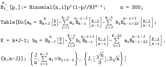
(for improved efficiency, we use only the relevant range of J values).

The program takes over one minute to execute; the results are displayed in Figure 3.

We can easily interpolate values of the corresponding table to convert it into a continuous function, thereby finding any desired value to a sufficient accuracy.

The main problem with this algorithm lies in its execution time, which increases (like most matrix-based computation) with roughly the third power of n. This makes the current approach rather prohibitive when dealing with samples consisting of thousands of observations.

In this context it is fair to mention that none of our programs have been optimized for run-time efficiency; even though some improvement in this regard is definitely possible, we do not believe that it would substantially change our general conclusions.

Figure 3. Pr(D₃₀₀ > d).

3. Generating-Function Solution

We now present an alternate way of building the same (discretized, but otherwise exact) solution. We start by defining the following function of two integer arguments

${\mathfrak{p}}_j^i\stackrel{\text{def}}{=}\frac{i^{i+j}}{\left(i+j\right)\mathrm{<mo>\; !\; </mo>}}$ (11)

Note that, when $i+j$ is negative (i is always positive), ${\mathfrak{p}}_j^i$ is equal to 0.

Claim 2. The binomial probability ${\mathbb{B}}_i^n\left(\frac{k}{n}\right)$ can be expressed in terms of three such $\mathfrak{p}$ functions, as follows

${\mathbb{B}}_i^n\left(\frac{k}{m}\right)=\frac{{\mathfrak{p}}_{i-k}^k\cdot {\mathfrak{p}}_{n-i-m+k}^{m-k}}{{\mathfrak{p}}_{n-m}^m}$ (12)

Proof.

${\mathbb{B}}_i^n\left(\frac{k}{m}\right)=\frac{n\mathrm{<mo>\; !\; </mo>}}{i\mathrm{<mo>\; !\; </mo>}\left(n-i\right)\mathrm{<mo>\; !\; </mo>}}{\left(\frac{k}{m}\right)}^i{\left(\frac{m-k}{m}\right)}^{n-i}=\frac{\frac{k^i}{i\mathrm{<mo>\; !\; </mo>}}\cdot \frac{{\left(m-k\right)}^{n-i}}{\left(n-i\right)\mathrm{<mo>\; !\; </mo>}}}{\frac{m^n}{n\mathrm{<mo>\; !\; </mo>}}}$ (13)

■

Note that $\mathbb{B}$ has the value of 0 whenever the number of successes (the subscript) is either negative or bigger than n (the superscript). Similarly, ${\mathbb{B}}_0^0$ is always equal to 1.

3.1. Modified Equations

The new function (11) enables us to express (7) and (9) in the following manner:

$\frac{{\mathfrak{p}}_J^k\cdot {\mathfrak{p}}_{-J}^{n-k}}{{\mathfrak{p}}_0^n}={\displaystyle \underset{i=1}{\overset{k}{\sum }}}Pr\left(A_i\right)\cdot \frac{{\mathfrak{p}}_0^{k-i}\cdot {\mathfrak{p}}_{-J}^{n-k}}{{\mathfrak{p}}_{-J}^{n-i}}+{\displaystyle \underset{i=J}{\overset{k-1}{\sum }}}Pr\left(B_i\right)\cdot \frac{{\mathfrak{p}}_{2J}^{k-i}\cdot {\mathfrak{p}}_{-J}^{n-k}}{{\mathfrak{p}}_J^{n-i}}$ (14)

and

$\frac{{\mathfrak{p}}_{-J}^k\cdot {\mathfrak{p}}_J^{n-k}}{{\mathfrak{p}}_0^n}={\displaystyle \underset{i=1}{\overset{k-1}{\sum }}}Pr\left(A_i\right)\cdot \frac{{\mathfrak{p}}_{-2J}^{k-i}\cdot {\mathfrak{p}}_J^{n-k}}{{\mathfrak{p}}_{-J}^{n-i}}+{\displaystyle \underset{i=J}{\overset{k}{\sum }}}Pr\left(B_i\right)\cdot \frac{{\mathfrak{p}}_0^{k-i}\cdot {\mathfrak{p}}_J^{n-k}}{{\mathfrak{p}}_J^{n-i}}$ (15)

respectively.

Cancelling ${\mathfrak{p}}_{-J}^{n-k}$ in each term of (14) and multiplying by ${\mathfrak{p}}_0^n$ yields

${\mathfrak{p}}_J^k={\displaystyle \underset{i=1}{\overset{k}{\sum }}}\frac{{\mathfrak{p}}_0^n}{{\mathfrak{p}}_{-J}^{n-i}}Pr\left(A_i\right)\cdot {\mathfrak{p}}_0^{k-i}+{\displaystyle \underset{i=J}{\overset{k-1}{\sum }}}\frac{{\mathfrak{p}}_0^n}{{\mathfrak{p}}_J^{n-i}}Pr\left(B_i\right)\cdot {\mathfrak{p}}_{2J}^{k-i}$ (16)

which can be written as

${\mathfrak{p}}_J^k={\displaystyle \underset{i=1}{\overset{k}{\sum }}}{a}_i\cdot {\mathfrak{p}}_0^{k-i}+{\displaystyle \underset{i=J}{\overset{k-1}{\sum }}}{b}_i\cdot {\mathfrak{p}}_{2J}^{k-i}$ (17)

(for any positive integer k), by defining

$a_i\stackrel{\text{def}}{=}\frac{{\mathfrak{p}}_0^n}{{\mathfrak{p}}_{-J}^{n-i}}Pr\left(A_i\right)$ (18)

and

$b_i\stackrel{\text{def}}{=}\frac{{\mathfrak{p}}_0^n}{{\mathfrak{p}}_J^{n-i}}Pr\left(B_i\right)$ (19)

Note that n has disappeared from (17), making $a_i$ and $b_i$ potentially infinite sequences (consider letting n have any positive value; in that sense $a_i$ is well defined for any i from 1 to $\infty$ and $b_i$ for any i from J to $\infty$ ). Once we solve for these two sequences, converting them back to $Pr\left(A_i\right)$ and $Pr\left(B_i\right)$ for any specific value of n is a simple task; this approach thus effectively deals with all n at the same time!

Similarly modifying (15) results in

${\mathfrak{p}}_{-J}^k={\displaystyle \underset{i=1}{\overset{k-1}{\sum }}}{a}_i\cdot {\mathfrak{p}}_{-2J}^{k-i}+{\displaystyle \underset{i=J}{\overset{k}{\sum }}}{b}_i\cdot {\mathfrak{p}}_0^{k-i}$ (20)

(for any $k>J$ ), utilizing the previous definition of $a_i$ and $b_i$. The equations, together with (17), constitute an infinite set of linear equations for elements of the two sequences. To find the corresponding solution, we reach for a different mathematical tool.

3.2. Generating Functions

Let us introduce the following generating functions

$G_a\left(t\right)\stackrel{\text{def}}{=}{\displaystyle \underset{k=1}{\overset{\infty }{\sum }}}{a}_k\cdot t^k$ (21)

$G_b\left(t\right)\stackrel{\text{def}}{=}{\displaystyle \underset{k=1}{\overset{\infty }{\sum }}}{b}_k\cdot t^k$

$G_j\left(t\right)\stackrel{\text{def}}{=}{\delta }_{j\mathrm{,0}}+{\displaystyle \underset{k=1}{\overset{\infty }{\sum }}}{\mathfrak{p}}_j^k\cdot t^k$

where j is a non-negative integer, and ${\delta }_{j\mathrm{,0}}$ (Kronecker’s $\delta$ ) is equal to 1 when $j=0$, equal to 0 otherwise.

Multiplying (17) by $t^k$ and summing over k from 1 to $\infty$ yields

$G_J\left(t\right)=G_a\left(t\right)\cdot G_0\left(t\right)+G_b\left(t\right)\cdot G_{2J}\left(t\right)$ (Gj)

since ${\displaystyle {\sum }_{i=1}^k}{a}_i\cdot {\mathfrak{p}}_0^{k-i}$ is the coefficient of $t^k$ in the expansion of $G_a\left(t\right)\cdot G_0\left(t\right)$, and ${\displaystyle {\sum }_{i=J}^{k-1}}{b}_i\cdot {\mathfrak{p}}_{2J}^{k-i}$ is the coefficient of $t^k$ in the expansion of $G_b\left(t\right)\cdot G_{2J}\left(t\right)$ ; combining two sequences in this manner is called their convolution. Note the importance (for correctness of the $G_a\cdot G_0$ result) of including ${\delta }_{j\mathrm{,0}}$ in the definition of $G_0\left(t\right)$.

Similarly, it follows from (20) that

$G_{-J}\left(t\right)=G_a\left(t\right)\cdot G_{-2J}\left(t\right)+G_b\left(t\right)\cdot G_0\left(t\right)$ (22)

3.3. Resulting Solution

The last two (simple, linear) equations can be so easily solved for $G_a\left(t\right)$ and $G_b\left(t\right)$ that we do not even quote the answer.

Going back to a specific sample size n, we now need to find the value of (10), namely

$\frac{{\displaystyle {\sum }_{i=1}^{n-1}{a}_i\cdot {\mathfrak{p}}_{-J}^{n-i}}+{\displaystyle {\sum }_{i=1}^{n-1}{b}_i\cdot {\mathfrak{p}}_J^{n-i}}}{{\mathfrak{p}}_0^n}$ (23)

which follows from solving (18) and (19) for $Pr\left(A_i\right)$ and $Pr\left(B_i\right)$ respectively. The numerator of the last expression is clearly (by the same convolution argument) the coefficient of $t^n$ in the expansion of

$G_a\left(t\right)\cdot G_{-J}\left(t\right)+G_b\left(t\right)\cdot G_J\left(t\right)$ (24)

An important point is that, in actual computation, the G functions need to be expanded only up to and including the $t^n$ term, making them long but otherwise simple polynomials.

The algorithm to find $Pr\left(D_n>d_J\right)$ then requires us to build $G_0\left(t\right)$, $G_J\left(t\right)$, $G_{-J}\left(t\right)$, $G_{2J}\left(t\right)$ and $G_{-2J}\left(t\right)$, and Taylor-expand, up to the same $t^n$ term,

$G_D\left(t\right)\stackrel{\text{def}}{=}\frac{2G_0\left(t\right)G_J\left(t\right)G_{-J}\left(t\right)-G_{-J}{\left(t\right)}^2{G}_{2J}\left(t\right)-G_J{\left(t\right)}^2{G}_{-2J}\left(t\right)}{\left(G_0{\left(t\right)}^2-G_{2J}\left(t\right)G_{-2J}\left(t\right)\right)\cdot {\mathfrak{p}}_0^n}$ (25)

which is obtained by substituting the solution to (Gj) and (22) into (24), and further dividing by ${\mathfrak{p}}_0^n$ ; $\mathrm{Pr}\left(D_n>d_J\right)$ is then provided by the resulting coefficient of $t^n$.

Note that, based on the same expansion, we can get $\mathrm{Pr}\left(D_n>d_J\right)$ for any smaller n as well, just by correspondingly replacing the value of ${\mathfrak{p}}_0^n$. Nevertheless, the process still needs to be repeated with all relevant values of J.

The corresponding Mathematica code looks as follows:

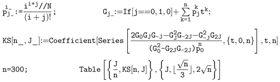
It produces results identical to those of the matrix-algebra algorithm, but has several advantages: the coding is somehow easier, it (almost) automatically yields results for any $n\le 300$ (not a part of our code) and it executes faster (taking about 17 seconds). Nevertheless, its run-time still increases with roughly the third power of n, thus preventing us from using it with a much larger value of n.

We now proceed to find several approximate solutions of increasing accuracy, all based on (25).

4. Asymptotic Solution

As we have seen, neither of the previous two solutions is very practical (and ultimately not even feasible) as the sample size increases. In that case, we have to switch to using an approximate (also referred to as asymptotic) solution.

Large-n Formulas

First, we must replace the old definition of ${\mathfrak{p}}_j^i$, namely (11), by

${\mathfrak{p}}_j^i\stackrel{\text{def}}{=}\frac{i^{i+j}\cdot {\text{e}}^{-i}}{\left(i+j\right)\mathrm{<mo>\; !\; </mo>}}$ (26)

Note that this does not affect (12), nor any of the subsequent formulas up to and including (25), since the various ${\text{e}}^{-i}$ factors always cancel out.

Also note that the definition can be easily extended to real (not just integer) arguments by using $\Gamma \left(i+j+1\right)$ in place of $\left(i+j\right)\mathrm{<mo>\; !\; </mo>}$, where $\Gamma$ denotes the usual gamma function.

1) Laplace representation

Note that, from now on, the summations defining the G functions in (21) stay infinite (no longer truncated to the first n terms only).

Consider a (rather general) generating function

$G\left(t\right)\stackrel{\text{def}}{=}{\displaystyle \underset{k=0}{\overset{\infty }{\sum }}}{p}_k\cdot t^k$ (27)

and an integer n ( $p$ may be implicitly a function of n as well as k); our goal is to find an approximation for $p_n$ as n increases.

After replacing k and t with two new variables x and s, thus

$k=n\cdot x$ (28)

$t=exp\left(-\frac{s}{n}\right)$

$G\left({\text{e}}^{-s/n}\right)$ becomes

${\displaystyle \underset{\begin{array}{c}x=0\\ \text{instepsof}\frac{1}{n}\end{array}}{\overset{\infty }{\sum }}}{p}_{x\cdot n}exp\left(-s\cdot x\right)$ (29)

Making the assumption that expanding $p_{x\cdot n}$ in powers of $\frac{1}{\sqrt{n}}$ results in

$p_{x\cdot n}=\frac{q\left(x\right)}{n}+O\left(\frac{1}{n^{3/2}}\right)\simeq \frac{q\left(x\right)}{n}$ (30)

(and our results do have this property), then (29) is approximately equal to

$\frac{1}{n}\cdot {\displaystyle \underset{\begin{array}{c}x=0\\ \text{instepsof}\frac{1}{n}\end{array}}{\overset{\infty }{\sum }}}q\left(x\right)exp\left(-s\cdot x\right)+\mathrm{<mi>\; </mi>}\cdots$ (31)

which, in the $n\to \infty$ limit, yields the following (large-n) approximation to $G\left({\text{e}}^{-s/n}\right)$ :

$L\left(s\right)\stackrel{\text{def}}{=}{\displaystyle {\int }_0^{\infty }}q\left(x\right)exp\left(-s\cdot x\right)\text{d}x$ (32)

Note that $L\left(s\right)$ is the so-called Laplace transform of $q\left(x\right)$ ; we call it the Laplace representation of G.

To find an approximate value of the coefficient of $t^n$ (i.e. $p_n\simeq \frac{q\left(1\right)}{n}$ ) of (27),

we need to find the so-called inverse Laplace transform (ILT) of $L\left(s\right)$ yielding the corresponding $q\left(x\right)$ then substitute 1 for x and divide by n (this is the gist of the technique of this section).

To improve this approximation, $q\left(x\right)$ itself and consequently $L\left(s\right)$ can be expanded in further powers of $\frac{1}{\sqrt{n}}$ (done eventually; but currently we concentrate on the $n\to \infty$ limit).

2) Approximating G_j

Let us now find Laplace representation of our $G_j$, i.e. the last line of (21), further divided by $\sqrt{n}$ (this is necessary to meet (30), yet it does not change (25) as long as ${\mathfrak{p}}_0^n$ of that formula is divided by $\sqrt{n}$ as well). To find the corresponding $q\left(x\right)$, we need the $n\to \infty$ limit of

$n\cdot \frac{{\mathfrak{p}}_j^k}{\sqrt{n}}=\frac{{\left(n\cdot x\right)}^{n\cdot x+j}exp\left(-n\cdot x\right)\sqrt{n}}{\left(n\cdot x+j\right)\mathrm{<mo>\; !\; </mo>}}$ (33)

To be able to reach a finite answer, j itself needs to be replaced by $z\sqrt{n}$ ; note that doing that with our J changes $\mathrm{Pr}\left(D_n>d_J\right)$ to $\mathrm{Pr}\left(\sqrt{n}\cdot D_n>z\right)$.

It happens to be easier to take the limit of the natural logarithm of (33), namely

$\left(x\cdot n+z\sqrt{n}\right)ln\left(x\cdot n\right)-x\cdot n+\frac{1}{2}lnn-ln\left(x\cdot n+z\sqrt{n}\right)\mathrm{<mo>\; !\; </mo>}$ (34)

instead.

With the help of the following version of Stirling’s formula (ignore its last term for the time being)

$ln\left(m\mathrm{<mo>\; !\; </mo>}\right)\simeq mlnm-m-\frac{1}{2}lnm+ln\sqrt{2\pi }+\frac{1}{12m}+\mathrm{<mi>\; </mi>}\cdots$ (35)

and of (we do not need the last two terms as yet)

$ln\left(x\cdot n+z\sqrt{n}\right)\simeq ln\left(x\cdot n\right)+\frac{z}{x\sqrt{n}}-\frac{z^2}{2x^{2}n}+\frac{z^3}{3x^3{n}^{3/2}}-\frac{z^4}{4x^4{n}^2}+\mathrm{<mi>\; </mi>}\cdots$ (36)

we get (this kind of tedious algebra is usually delegated to a computer)

$lnq\left(x\right)\simeq -\frac{z^2}{2x}-ln\sqrt{2\pi x}+\mathrm{<mi>\; </mi>}\cdots$ (37)

We thus end up with

$\frac{G_j\left({\text{e}}^{-s/n}\right)}{\sqrt{n}}\underset{n\to \infty }{\to }\frac{1}{\sqrt{2\pi }}{\displaystyle {\int }_0^{\infty }}\frac{exp\left(-\frac{z^2}{2x}-x\cdot s\right)}{\sqrt{x}}\text{d}x=\frac{exp\left(-\sqrt{2z^{2}s}\right)}{\sqrt{2s}}$ (38)

where $z=\frac{j}{\sqrt{n}}$ ; this follows from (32) and the following result:

Claim 3.

$I_v\stackrel{\text{def}}{=}{\displaystyle {\int }_0^{\infty }}\frac{exp\left(-\frac{v}{x}-x\cdot s\right)}{\sqrt{x}}\mathrm{<mi>\; </mi>}\text{d}x=\sqrt{\frac{\pi }{s}}\cdot exp\left(-2\sqrt{v\cdot s}\right)$ (39)

when v and s are positive

Proof. Since

$\frac{\text{d}{I}_v}{\text{d}v}={\displaystyle {\int }_0^{\infty }}\frac{exp\left(-\frac{v}{x}-x\cdot s\right)}{x^{3/2}}\mathrm{<mi>\; </mi>}\text{d}x$ (40)

and

$I_v={\displaystyle {\int }_0^{\infty }}\frac{exp\left(-s\cdot y-\frac{v}{y}\right)}{\sqrt{\frac{v}{s\cdot y}}}\cdot \frac{v}{s\cdot y^2}\mathrm{<mi>\; </mi>}\text{d}y=\sqrt{\frac{v}{s}}\cdot \frac{\text{d}{I}_v}{\text{d}v}$ (41)

after the $x=\frac{v}{s\cdot y}$ substitution. Solving the resulting simple differential equation for $I_v$ yields

$I_v=c\cdot exp\left(2\sqrt{v\cdot s}\right)$ (42)

where c is equal to

$I_0={\displaystyle {\int }_0^{\infty }}\frac{exp\left(-x\cdot s\right)}{\sqrt{x}}\text{d}x={\displaystyle {\int }_0^{\infty }}\frac{exp\left(-u^2\cdot s\right)}{u}\cdot 2u\text{d}u=\sqrt{\frac{\pi }{s}}$ (43)

the last being a well-known integral (related to Normal distribution). ■

To find the $n\to \infty$ limit of (25), we first evaluate the right hand side of (38) with $j=-2J\mathrm{,}-J\mathrm{,0},J$ and 2J, getting

$\frac{G_0\left({\text{e}}^{-s/n}\right)}{\sqrt{n}}\underset{n\to \infty }{\to }\frac{1}{\sqrt{2s}}$ (44)

$\frac{G_J\left({\text{e}}^{-s/n}\right)}{\sqrt{n}}=\frac{G_{-J}\left({\text{e}}^{-s/n}\right)}{\sqrt{n}}\underset{n\to \infty }{\to }\frac{exp\left(-z\sqrt{2s}\right)}{\sqrt{2s}}$

$\frac{G_{2J}\left({\text{e}}^{-s/n}\right)}{\sqrt{n}}=\frac{G_{-2J}\left({\text{e}}^{-s/n}\right)}{\sqrt{n}}\underset{n\to \infty }{\to }\frac{exp\left(-2z\sqrt{2s}\right)}{\sqrt{2s}}$

where $z=\frac{J}{\sqrt{n}}$ (always positive).

3) Approximating G_D

The corresponding Laplace representation of (25) further divided by n, let us denote it $L_{D\mathrm{<mo>\; /\; </mo>}n}\left(s\right)$, is then equal to

$\frac{2\cdot \frac{E}{2s\sqrt{2s}}-2\cdot \frac{E^2}{2s\sqrt{2s}}}{\left(\frac{1-E^2}{2s}\right)\cdot \frac{1}{\sqrt{2\pi }}}=\frac{2\cdot E}{1+E}\cdot \sqrt{\frac{2\pi }{2s}}=2\cdot \sqrt{\frac{2\pi }{2s}}\cdot {\displaystyle \underset{k=1}{\overset{\infty }{\sum }}}{\left(-1\right)}^{k-1}{E}^k$ (45)

where $E\stackrel{\text{def}}{=}\exp \left(-2z\sqrt{2s}\right)$. This is based on substituting the right-hand sides of (44) into (25), and on the following result:

$\underset{n\to \infty }{lim}\frac{{\mathfrak{p}}_0^n}{\sqrt{n}}\cdot n=\underset{n\to \infty }{lim}\frac{n^n{\text{e}}^{-n}\sqrt{n}}{n\mathrm{<mo>\; !\; </mo>}}=\frac{1}{\sqrt{2\pi }}$ (46)

(Stirling’s formula again); the last limit also makes it clear why we had to divide (25) by n: to ensure getting a finite result again.

We now need to find the $q_{D\mathrm{<mo>\; /\; </mo>}n}\left(x\right)$ function corresponding to (45), i.e. the latter’s ILT, and convert it to $p_n=\frac{q_{D\mathrm{<mo>\; /\; </mo>}n}\left(1\right)}{n}$ according to (30); this yields an approximation for the coefficient of $t^n$ in the expansion of (25), still divided by n. The ultimate answer to $Pr\left(\sqrt{n}{D}_n>z\right)$ is thus $\frac{q_{D\mathrm{<mo>\; /\; </mo>}n}\left(1\right)}{n}\cdot n=q_{D\mathrm{<mo>\; /\; </mo>}n}\left(1\right)$.

Since the ILT of

$\sqrt{\frac{\pi }{s}}\cdot E^k=\sqrt{\frac{\pi }{s}}\cdot \exp \left(-2kz\sqrt{2s}\right)$ (47)

(where k is a positive integer) is equal to

$\frac{exp\left(-\frac{2z^2{k}^2}{x}\right)}{\sqrt{x}}$ (48)

(this follows from (32) and (38), after replacing z by $z\cdot k$ ), its contribution to $q_{D\mathrm{<mo>\; /\; </mo>}n}\left(1\right)$ is

$exp\left(-2z^2{k}^2\right)$ (49)

Applied to the last line of (45), this leads to

$Pr\left(\sqrt{n}{D}_n>z\right)\underset{n\to \infty }{\to }2{\mathbb{T}}_0\left(z\right)$ (50)

or, equivalently,

$Pr\left(\sqrt{n}{D}_n\le z\right)\simeq 1-2{\mathbb{T}}_0\left(z\right)$ (51)

where

${\mathbb{T}}_0\left(z\right)\stackrel{\text{def}}{=}{\displaystyle \underset{k=1}{\overset{\infty }{\sum }}}{\left(-1\right)}^{k-1}exp\left(-2z^2{k}^2\right)$ (52)

Note that the error of this approximation is of the $O\left(\frac{1}{\sqrt{n}}\right)$ type, which means that it decreases, roughly (since there are also terms proportional to $\frac{1}{n}$, $\frac{1}{n^{3/2}}$, etc.), with $\frac{1}{\sqrt{n}}$. Also note that the right hand side of (51) can be easily evaluated by calling a special function readily available (under various names) with most symbolic programming languages, for example “JacobiTheta4(0, exp(−2∙z²))” of Maple or “EllipticTheta[4, 0, Exp[−2z²]]” of Mathematica.

The last formula has several advantages over the approach of the previous two sections: firstly, it is easy and practically instantaneous to evaluate (the infinite series converges rather quickly only between 2 and 10 terms are required to reach a sufficient accuracy when $0.3<z$ the CDF is practically zero otherwise), secondly, it is automatically a continuous function of z (no need to interpolate), and finally, it provides an approximate distribution of $\sqrt{n}{D}_n$ for all values of n (the larger the n, the better the approximation).

But a big disappointment is the formula’s accuracy, becoming adequate only when the sample size n reaches thousands of observations; for smaller samples, an improvement is clearly necessary. To demonstrate this, we have computed the difference between the exact and approximate CDF when $n=300$ ; see Figure 4, which is in agreement with a similar graph of [2].

We can see that the maximum possible error of the approximation is over 1.5% (when computing the probability of $D_{300}>0.046$ ); errors of this size are generally not considered acceptable.

5. High-Accuracy Solution

Results of this section were obtained (in a slightly different form, and building on previously published results) by [5] and further expounded by a more accessible [6]; their method is based on expanding (in powers of $\frac{1}{\sqrt{n}}$ ) the matrix-algebra solution. Here we present an alternate approach, similarly expanding the generating-function solution instead; this appears an easier way of deriving the individual $\frac{1}{\sqrt{n}}$ and $\frac{1}{n}$ -proportional corrections to (50). We should mention that the cited articles include the $\frac{1}{n^{3/2}}$ -proportional correction as well; it would not be difficult to extend our results in the same manner, if deemed beneficial.

To improve accuracy of our previous asymptotic solution, (34) and, consequently, (38) have to be extended by extra $\frac{1}{\sqrt{n}}$ and $\frac{1}{n}$ -proportional terms (note that (35) and (36) were already presented in this extended form), getting

$\begin{array}{l}\frac{G_j\left({\text{e}}^{-s/n}\right)}{\sqrt{n}}\\ \simeq {\displaystyle {\int }_0^{\infty }}\frac{exp\left(-\frac{z^2}{2x}-s\cdot x\right)\cdot \left(1+\frac{z^3-3z\cdot x}{6x^2\sqrt{n}}+\frac{z^6-12z^{4}x+27z^2{x}^2-6x^3}{72x^{4}n}+\mathrm{<mi>\; </mi>}\cdots \right)}{\sqrt{2\pi \cdot x}}\text{d}x\\ =\frac{exp\left(-\sqrt{2z^{2}s}\right)}{\sqrt{2s}}\cdot \left(1+\frac{s\cdot z\mp \sqrt{2s}}{3\sqrt{n}}+\frac{z^2{s}^2-3\sqrt{2z^2{s}^3}+3s}{18n}+\mathrm{<mi>\; </mi>}\cdots \right)\end{array}$ (53)

where the $\mp$ sign corresponds to a positive (negative) $z\stackrel{\text{def}}{=}\frac{j}{\sqrt{n}}$, respectively. The corresponding tedius algebra is usually delegated to a computer (it is no longer feasible to show all the details here), the necessary integrals are found by differentiating each side of the equation in (38) with respect to z², from one up to four times.

The last expression represents an excellent approximation to the G functions of (44), with the exception of

$G_0\left({\text{e}}^{-s/n}\right)\stackrel{\text{def}}{=}{\displaystyle \underset{k=0}{\overset{\infty }{\sum }}}{\mathfrak{p}}_0^k\cdot exp\left(-\frac{ks}{n}\right)$ (54)

Figure 4. Error of asymptotic solution (n = 300).

which now requires a different approach.

Claim 4.

$\frac{G_0\left({\text{e}}^{-s/n}\right)}{\sqrt{n}}\simeq \frac{1}{\sqrt{2s}}+\frac{1}{3\sqrt{n}}+\frac{\sqrt{2s}}{12n}+\mathrm{<mi>\; </mi>}\cdots$ (55)

Proof. The following elegant proof has been suggested by [7].

It is well known that the value of Lambert $W\left(z\right)$ function is defined as a solution to $w{\text{e}}^w=z$, and that its Taylor expansion is given by

${\displaystyle \underset{k=1}{\overset{\infty }{\sum }}}\frac{{\left(-k\right)}^{k-1}}{k\mathrm{<mo>\; !\; </mo>}}{z}^k$ (56)

implying that

${\displaystyle \underset{k=0}{\overset{\infty }{\sum }}}\frac{k^k}{k\mathrm{<mo>\; !\; </mo>}}{\text{e}}^{-k\left(1+\lambda \right)}=1+\frac{\text{d}}{\text{d}\lambda }W\left(-{\text{e}}^{-\lambda -1}\right)$ (57)

■

Differentiating

$w{\text{e}}^w=-{\text{e}}^{-\lambda -1}$ (58)

with respect to $\lambda$, cancelling ${\text{e}}^w$, and solving for $\frac{\text{d}w}{\text{d}\lambda }$ yields

$\frac{\text{d}w}{\text{d}\lambda }=-\frac{w}{1+w}$ (59)

implying that

${\displaystyle \underset{k=0}{\overset{\infty }{\sum }}}\frac{k^k}{k\mathrm{<mo>\; !\; </mo>}}{\text{e}}^{-k\left(1+\lambda \right)}=\frac{1}{1+w}\stackrel{\text{def}}{=}\frac{1}{u}$ (60)

where u (being equal to $1+w$ ) is now the solution of

$\left(u-1\right){\text{e}}^u=-{\text{e}}^{-\lambda }$ (61)

rather than (58). Solving the last equation for $\lambda$ and expanding the answer in powers of u results in

$\lambda =\frac{u^2}{2}+\frac{u^3}{3}+\frac{u^4}{4}+\cdots$ (62)

Inverting the last power series (which can be easily done to any number of terms) yields the following expansion:

$u=\sqrt{2\lambda }-\frac{2\lambda }{3n}+\frac{{\left(2\lambda \right)}^{3/2}}{36}+\cdots$ (63)

Similarly expanding $\frac{1}{u}$, replacing $\lambda$ by $\frac{s}{n}$ and further dividing by $\sqrt{n}$ proves our claim.

Having achieved more accurate approximation for all our G functions, and with the following extension of (46)

$\frac{n^n{\text{e}}^{-n}\sqrt{n}}{n\mathrm{<mo>\; !\; </mo>}}\simeq \frac{1}{\sqrt{2\pi }}\cdot \left(1-\frac{1}{12n}+\mathrm{<mi>\; </mi>}\cdots \right)$ (64)

we can now complete the corresponding refinement of (45) by substituting all these expansions into (25), further divided by n. This results in

$\begin{array}{c}{L}_{D\mathrm{<mo>\; /\; </mo>}n}\left(s\right)\simeq \sqrt{2\pi }\cdot \frac{2E_{+}}{1+E_{+}}\cdot \frac{1}{\sqrt{2s}}+\frac{\sqrt{2\pi }}{n}\cdot \frac{E}{6\left(1+E\right)}\cdot \frac{1}{\sqrt{2s}}\\ +\frac{\sqrt{2\pi }}{n}\cdot \left(\frac{E}{9\left(1+E\right)}-\frac{E}{18\left(1-E\right)}\right)\sqrt{2s}-\frac{\sqrt{2\pi }}{n}\cdot \frac{z\cdot E}{9{\left(1+E\right)}^2}\cdot 2s+\mathrm{<mi>\; </mi>}\cdots \end{array}$ (65)

The last formula consists of two types of corrections: replacing E by

$E_{+}\stackrel{\text{def}}{=}\exp \left(-2\left(z+\frac{1}{6\sqrt{n}}\right)\sqrt{2s}\right)$ (66)

in its leading term removes the $\frac{1}{\sqrt{n}}$ -proportional error of (45); the remaining terms similarly represent the $\frac{1}{n}$ -proportional correction; the error of (65) is thus of the $O\left(\frac{1}{n^{3/2}}\right)$ type.

Note that

$E_{+}\simeq E\left(1+\frac{\sqrt{2s}}{3\sqrt{n}}+\frac{s}{9n}+\mathrm{<mi>\; </mi>}\cdots \right)$ (67)

enables us to express (65) in terms of E only; this is needed for its explicit verification (something we leave to a computer).

What we must do now is to convert (65) to the corresponding $q_{D\mathrm{<mo>\; /\; </mo>}n}\left(1\right)$, thus approximating the coefficient of $t^n$ in the expansion of (25). We already possess the answer for the first two terms of (65), which are both identical to (45), except that ${\mathbb{T}}_0\left(z\right)$ needs to be replaced by ${\mathbb{T}}_0\left(z+\frac{1}{6\sqrt{n}}\right)$ in the first case, and divided by 12 in the second one.

To convert the remaining terms of (65) to their $q_{D\mathrm{<mo>\; /\; </mo>}n}\left(1\right)$ contribution, we must first expand them in powers of E, then take the ILT of individual terms of these expansions, and finally set x equal to 1; the following table helps with the last two steps:

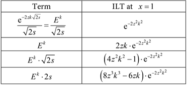(68)

(the first row has already been proven; the remaining three follow by differentiating both of its sides with respect to zk (taken as a single variable), up to three times).

This results in the following replacement

$\sqrt{2\pi }\cdot \frac{E}{1+E}\cdot \sqrt{2s}\to {\displaystyle \underset{k=1}{\overset{\infty }{\sum }}}{\left(-1\right)}^{k-1}{\text{e}}^{-2z^2{k}^2}\left(4k^2{z}^2-1\right)$

$\sqrt{2\pi }\cdot \frac{E}{1-E}\cdot \sqrt{2s}\to {\displaystyle \underset{k=1}{\overset{\infty }{\sum }}}{\text{e}}^{-2z^2{k}^2}\left(4k^2{z}^2-1\right)$ (69)

$\sqrt{2\pi }\cdot \frac{zE}{{\left(1+E\right)}^2}\cdot 2s\to z{\displaystyle \underset{k=1}{\overset{\infty }{\sum }}}\left(\begin{array}{c}-2\\ k-1\end{array}\right){\text{e}}^{-2z^2{k}^2}\left(8k^3{z}^3-6kz\right)$

where all three series are still fast-converging. Note that the binomial coefficient of the last sum equals to ${\left(-1\right)}^{k-1}k$.

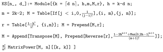
We can then present our final answer for $\mathrm{Pr}\left(\sqrt{n}{D}_n>z\right)$ in the manner of the following Mathematica code; the resulting KS function can then compute (practically instantaneously) this probability for any n and z.

The resulting improvement in accuracy over the previous, asymptotic approximation is quite dramatic; Figure 5 again displays the difference between the exact and approximate CDF of $D_{300}$.

This time, the maximum error has been reduced to an impressive 0.0036%, this happens when computing $\mathrm{Pr}\left(0.027<D_{300}<0.0475\right)$ ; note that potential errors become substantially smaller in the right hand tail (the critical part) of the distribution. Most importantly, when the same computation is repeated with $n=10$, the corresponding graph indicates that errors of the new approximation

Figure 5. Error of high-accuracy solution (n = 300).

can never exceed 0.20%; such an accuracy would be normally considered quite adequate (approximating Student’s $t_{30}$ by Normal distribution can yield an error almost as large as 1%).

As mentioned already, the approximation of $Pr\left(\sqrt{n}{D}_n>z\right)$ can be made even more accurate by adding, to the current expansion, the following extra $n^{-3/2}$ -proportional correction

$\begin{array}{l}+\frac{z}{27n^{3/2}}{\displaystyle \underset{k=1}{\overset{\infty }{\sum }}}{\left(-1\right)}^{k-1}\exp \left(-2z^2{k}^2\right)\\ \times k^2\left\{\left(k^2+\frac{107}{5}+3{\left(-1\right)}^k\right)\cdot \left(1-\frac{4}{3}{k}^2{z}^2\right)-\frac{78}{5}+16k^4{z}^4\right\}\end{array}$ (70)

At $n=300$, this reduces the corresponding error by a factor of 4; nevertheless, from a practical point of view, such high accuracy is hardly ever required. Furthermore, the new term reduces the maximum error of the $n=10$ result from the previous 0.17% only to 0.10%; even though this represents an undisputable improvement, it is achieved at the expense of increased complexity. Note that adding higher ( $\frac{1}{n^2}$ -proportional, etc.) terms of the expansion would no longer (at $n=10$ ) improve its accuracy, since the expansion starts diverging (a phenomenon also observed with, and effectively inherited from, the Stirling expansion); this happens quite early when n is small (and, when n is large, higher accuracy is no longer needed).

When simplicity, speed of computation, and reasonable accuracy are desired in a single formula, the next section presents a possible solution.

Final Simplification

We have already seen that the $\frac{1}{\sqrt{n}}$ -proportional error is removed by the following trivial modification of (50)

$Pr\left(\sqrt{n}{D}_n\le z\right)=1-2{\mathbb{T}}_0\left(z+\frac{1}{6\sqrt{n}}\right)$ (71)

Note that this amounts only to a slight shift of the whole curve to the left, but leaves us with a full $O\left(\frac{1}{n}\right)$ -type error.

When willing to compromise, [8] has taken this one step further: it is possible to show that, by extending the argument of ${\mathbb{T}}_0$ to

$z+\frac{1}{6\sqrt{n}}+\frac{z-1}{4n}$ (72)

yields results which are very close to achieving the full $\frac{1}{n}$ -proportional correction of (65) as well; this is a fortuitous empirical results which can be easily verified computationally (when $n=10$, the maximum error of the last approximation increases to 0.27%, for $n=300$ it goes up to 0.0096% still practically negligible).

6. Conclusions and Summary

In this article, we hope to have met two goals:

• explaining, in every possible detail, the traditional derivations (two of them yielding exact results, several of them being approximate) of the $D_n$ distribution,

• proposing the following simple modification of the commonly used formula:

$Pr\left(\sqrt{n}{D}_n\le z\right)\simeq 1+\mathrm{2\; <mi>\; </mi>}{\displaystyle \underset{k=1}{\overset{\infty }{\sum }}}{\left(-1\right)}^{k}exp\left(-2{\left(z+\frac{1}{6\sqrt{n}}+\frac{z-1}{4n}\right)}^2{k}^2\right)$ (73)

making it accurate enough to be used as a practical substitute for exact results even with relatively small samples. Furthermore, the right hand side of this formula can be easily evaluated by computer software (see the comment following (52)).

Appendix

The following Mathematica function computes the exact $Pr\left(D_n\le d\right)$ for any value of d; using it to produce a full graph of the corresponding CDF will work only for a sample size not much bigger than 700, since the algorithm’s computational time increases exponentially with not only n, but also with increasing values of d.

Nevertheless, computing only a single value of this function (such as a P value of an observed $D_n$ ) becomes feasible even for a substantially bigger sample size; for example: typing KS[3000, 0.031467] results in 0.994855, taking about 13 seconds on an average computer. Increasing n any further would necessitate switching to one of the (at that point, extremely accurate) approximations of our article.

Conflicts of Interest

The author declares no conflicts of interest regarding the publication of this paper.

References

[1]	Durbin, J. (1973) Distribution Theory for Tests Based on the Sample Distribution Function. Society for Industrial and Applied Mathematics, Philadelphia. https://doi.org/10.1137/1.9781611970586
[2]	Marsaglia, G., Tsang, W.W. and Wang, J. (2003) Evaluating Kolmogorov’s Distribution. Journal of Statistical Software, 8, 1-4. https://doi.org/10.18637/jss.v008.i18
[3]	Feller, W. (1948) On the Kolmogorov-Smirnov Limit Theorems for Empirical Distributions. Annals of Mathematical Statistics, 19, 177-189. https://doi.org/10.1214/aoms/1177730243
[4]	Kendall, M.G. and Stuart, A. (1973) The Advanced Theory of Statistics. Vol. 2, Hafner Publishing Company, New York, 468-477.
[5]	Chang, L.C. (1956) On the Exact Distribution of the Statistics of A. N. Kolmogorov and Their Asymptotic Expansion. Acta Mathematica Sinica, 6, 55-81.
[6]	Pelz, W. and Good, I.J. (1976) Approximation the Lower Tail Areas of the Kolmogorov-Smirnov One Sample Statistic. Journal of he Royal Statistical Society, Series B, 38, 152-156. https://doi.org/10.1111/j.2517-6161.1976.tb01579.x
[7]	https://math.stackexchange.com/q/3247174
[8]	Vrbik, J. (2018) Small-Sample Corrections to Kolmogorov-Smirnov Test Statistic. Pioneer Journal of Theoretical and Applied Statistics, 15, 15-23.