A Smoothing Penalty Function Method for the Constrained Optimization Problem ()
1. Introduction
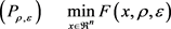
Many problems in industry design, management science and economics can be modeled as the following constrained optimization problem:
(1)
where
are continuously differentiable functions. Let
be the feasible solution set, that is,
. Here we assume that
is nonempty.
The penalty function methods based on various penalty functions have been proposed to solve problem (P) in the literatures. One of the popular penalty functions is the quadratic penalty function with the form
(2)
where
is a penalty parameter. Clearly,
is continuously differentiable, but is not an exact penalty function. In Zangwill [1], an exact penalty function was defined as
(3)
The corresponding penalty problem is
(4)
We say that
is an exact penalty function for Problem (P) partly because it satisfies one of the main characteristics of exactness, that is, under some constraint qualifications, there exists a sufficiently large
such that for each
, the optimal solutions of Problem (
) are all the feasible solutions of Problem (P), therefore, they are all the optimal solution of (P) (Di Pillo [2], Han [3] ).
The obvious difficulty with the exact penalty functions is that it is nondifferentiable, which prevents the use of efficient minimization methods that are based on Gradient-type or Newton-type algorithms, and may cause some numerical instability problems in its implementation. In practice, an approximately optimal solution to (P) is often only needed. Differentiable approximations to the exact penalty function have been obtained in different contexts such as in BeaTal and Teboulle [4], Herty et al. [5] and Pinar and Zenios [6]. Penalty methods based on functions of this class were studied by Auslender, Cominetti and Haddou [7] for convex and linear programming problems, and by Gonzaga and Castillo [8] for nonlinear inequality constrained optimization problems, respectively. In Xu et al. [9] and Lian [10], smoothing penalty functions are proposed for nonlinear inequality constrained optimization problems. This kind of functions is also described by Chen and Mangasarian [11] who constructed them by integrating probability distributions to study complementarity problems, by Herty et al. [5] to study the optimization problems with box and equality constraints, and by Wu et al. [12] to study global optimization problem. Meng et al. [13] propose two smoothing penalty functions to the exact penalty function
(5)
In Wu et al. [14] and Lian [15], some smoothing techniques for (5) are also given.
Moreover, smoothed penalty methods can be applied to solve optimization problems with large scale such as network-structured problems and minimax problems in [6], and traffic flow network models in [5].
In this paper, we consider another simpler method for smoothing the exact penalty function
, and construct the corresponding smoothed penalty problem. We show that our smooth penalty function can approximate
well and has better smoothness. Based on our smooth penalty function, we give for (P) a simple smoothed penalty algorithm which is different from the existing literature in that the convergence of it can be obtained without the compactness of the feasible region of (P). We also give an approximate algorithm which enjoys some convergence under mild conditions.
The rest of this paper is organized as follows. In Section 2, we propose a method for smoothing the
exact penalty function (3). The approximation function we give is convex and smooth. We give some error estimates among the optimal objective function values of the smoothed penalty problem, of the nonsmooth penalty problem and of the original constrained optimization problem. In Section 3, we present an algorithm to compute a solution to (P) based on our smooth penalty function and show the convergence of the algorithm. In particular, we give an approximate algorithm. Some computational aspects are discussed and some experiment results are given in Section 4.
2. A Smooth Penalty Function
We define a function
:
(6)
given any
.
Let
, for any
. It is easy to show that
.
The function
is different from the function
given in [16] since here we use two parameters
and . The function
  has the following abstractive properties.
(I)  is at least twice continuously differentiable in t for
 . In fact, we have that
 (7)
(7)
and
 (8)
(8)
(II)  is convex and monotonically increasing in t for any given
 .
.
Property (II) can follow from (I) immediately.
Note that . Consider the penalty function for (P) given by
 (9)
(9)
where  is a penalty parameter. Clearly,
  is at least twice continuously differentiable in any
 , if
, if  are all at least twice continuously differentiable, and
  is convex, if
  are all convex functions.
The corresponding penalty problem to  is given as follows:
 .
.
Since ![]() for any given
for any given![]() , we will first study the relationship between (
, we will first study the relationship between (![]() ) and (
) and (![]() ).
).
The following Lemma is easily to prove.
Lemma 2.1 For any given![]() , and
, and![]() ,
,
![]()
Two direct results of Lemma 2.1 are given as follows.
Theorem 2.1 Let ![]() be a sequence of positive numbers and assume
be a sequence of positive numbers and assume ![]() is a solution to
is a solution to ![]() for some given
for some given![]() . Let
. Let ![]() be an accumulating point of the sequence
be an accumulating point of the sequence![]() , then
, then ![]() is an optimal solution to
is an optimal solution to![]() .
.
Theorem 2.2 Let ![]() be an optimal solution of (
be an optimal solution of (![]() ) and
) and ![]() an optimal solution of (
an optimal solution of (![]() ). Then
). Then
![]()
It follows from this conclusion that ![]() can approximate
can approximate ![]() well.
well.
Theorem 2.1 and Theorem 2.2 show that an approximate solution to (![]() ) is also an approximate solution to (
) is also an approximate solution to (![]() ) when
) when ![]() is sufficiently small.
is sufficiently small.
Definition 2.1 A point ![]() is a
is a ![]() -feasible solution or a
-feasible solution or a ![]() -solution if,
-solution if,
![]()
Under this definition, we get the following result.
Theorem 2.3 Let ![]() be an optimal solution of (
be an optimal solution of (![]() ) and
) and ![]() an optimal solution of (
an optimal solution of (![]() ). Furthermore, let
). Furthermore, let ![]() be feasible to (P) and
be feasible to (P) and ![]() be
be ![]() -feasible to (P). Then,
-feasible to (P). Then,
![]()
Proof Since ![]() is
is ![]() -feasible to (P), then
-feasible to (P), then
![]()
![]() (10)
(10)
Since ![]() is an optimal solution to (P), we have
is an optimal solution to (P), we have
![]()
Then by Theorem 2.2, we get
![]()
Thus,
![]()
Therefore, by (10), we obtain that
![]()
This completes the proof.
By Theorem 2.3, if an approximate optimal solution of (![]() ) is
) is ![]() -feasible, then it is an approximate optimal solution of (P).
-feasible, then it is an approximate optimal solution of (P).
For ![]() penalty function
penalty function![]() , there is a well known result of its exactness (see [3] ):
, there is a well known result of its exactness (see [3] ):
(*) There exists a![]() , such that whenever
, such that whenever![]() , each optimal solution of
, each optimal solution of ![]() is also an optimal solution of (P).
is also an optimal solution of (P).
From the above conclusion, we can get the following result.
Theorem 2.4 For the constant ![]() in (*), let
in (*), let ![]() be an optimal solution of (
be an optimal solution of (![]() ). Suppose that for any
). Suppose that for any![]() ,
, ![]() is an optimal solution of (
is an optimal solution of (![]() ) where
) where![]() , then
, then ![]() is a
is a ![]() - feasible solution of (P).
- feasible solution of (P).
Proof Suppose the contrary that the theorem does not hold, then there exists a![]() , and
, and![]() , such that
, such that ![]() is an optimal solution for (
is an optimal solution for (![]() ), and the set
), and the set ![]() is not empty.
is not empty.
Since ![]() is an optimal solution for (
is an optimal solution for (![]() ) when
) when![]() , then for any
, then for any![]() , it holds that
, it holds that
![]() (11)
(11)
Because ![]() is an optimal solution of (
is an optimal solution of (![]() ),
),![]() is a feasible solution of (P). Therefore, we have that
is a feasible solution of (P). Therefore, we have that
![]()
On the other side,
![]()
![]()
which contradicts (11).
Theorem 2.4 implies that any optimal solution of the smoothed penalty problem is an approximately feasible solution of (P).
3. The Smoothed Penalty Algorithm
In this section, we give an algorithm based on the smoothed penalty function given in Section 2 to solve the nonlinear programming problem (P).
For![]() , we denote
, we denote
![]()
![]()
![]()
![]()
![]()
For Problem (P), let![]() , for some
, for some![]() . We consider the following algorithm.
. We consider the following algorithm.
Algorithm 3.1
Step 1. Given![]() , and
, and![]() , let
, let![]() , go to Step 2.
, go to Step 2.
Step 2. Take ![]() as the initial point, and compute
as the initial point, and compute
![]() (12)
(12)
Step 3. Let![]() , and
, and
![]() (13)
(13)
Let![]() , go to Step 2.
, go to Step 2.
We now give a convergence result for this algorithm under some mild conditions. First, we give the following assumption.
(A1) For any![]() ,
, ![]() , the set
, the set![]() .
.
By this assumption, we obtain the following lemma firstly.
Lemma 3.1 Suppose that (A1) holds. Let ![]() be the sequence generated by Algorithm 3.1. Then there exists a natural number
be the sequence generated by Algorithm 3.1. Then there exists a natural number![]() , such that for any
, such that for any![]() ,
,
![]()
Proof Suppose the contrary that there exists a subset![]() , such that for any k,
, such that for any k, ![]() , and
, and
![]()
Then there exists![]() , such that for any
, such that for any![]() ,
, ![]() , where
, where ![]() is given in Theorem 2.4. Therefore, by Theorem 2.4, when
is given in Theorem 2.4. Therefore, by Theorem 2.4, when![]() , it holds that
, it holds that
![]()
This contradicts![]() .
.
Remark 3.1 From Lemma 3.1 we know that ![]() remains unchanged after finite iterations.
remains unchanged after finite iterations.
Lemma 3.2 Suppose that (A1) holds. Let ![]() be the sequence generated by Algorithm 3.1, and
be the sequence generated by Algorithm 3.1, and ![]() be any limit point of
be any limit point of![]() . Then
. Then
![]()
Lemma 3.3 Suppose that (A1) holds. Let ![]() be the sequence generated by Algorithm 3.1. Then for any k,
be the sequence generated by Algorithm 3.1. Then for any k,
![]() (14)
(14)
From Lemma 3.2 and Lemma 3.3, we have the following theorem.
Theorem 3.1 Suppose that (A1) holds. Let ![]() be the sequence generated by Algorithm 3.1. If
be the sequence generated by Algorithm 3.1. If ![]() is any limit point of
is any limit point of![]() , then
, then ![]() is the optimal solution of (P).
is the optimal solution of (P).
Before giving another conclusion, we need the following assumption.
(A2) The function ![]() with respect to
with respect to ![]() is lower semi-continuous at
is lower semi-continuous at![]() .
.
Theorem 3.2 Suppose that (A1) and (A2) holds. Let ![]() be the sequence generated by Algorithm 3.1. Then
be the sequence generated by Algorithm 3.1. Then
![]()
Proof By Lemma 3.1, there exists![]() , such that for any
, such that for any![]() ,
,![]() . Thus,
. Thus,
![]()
Therefore,
![]()
From Assumption (A2), we know that![]() . Therefore,
. Therefore,
![]() (15)
(15)
On the other side, by Lemma 3.3, when![]() , we have
, we have
![]()
Then
![]() (16)
(16)
Therefore, from (15) and (16),
![]()
Therefore,
![]()
The above theorem is different from the conventional conclusion in other literatures with respect to the convergence of penalty method.
In the following we give an approximate smoothed penalty algorithm for Problem (P).
Algorithm 3.2
Step 1. Let![]() ,
,![]() . Given
. Given![]() , and
, and![]() , let
, let![]() , go to Step 2.
, go to Step 2.
Step 2. Take ![]() as the initial point, and compute
as the initial point, and compute
![]()
Step 3. If ![]() is an
is an ![]() -feasible solution of (P), and
-feasible solution of (P), and![]() , then stop. Otherwise, update
, then stop. Otherwise, update ![]() and
and ![]() by applying the following rules:
by applying the following rules:
if ![]() is an
is an ![]() -feasible solution of (P), and
-feasible solution of (P), and![]() , let
, let![]() , and
, and
![]() ;
;
if ![]() is not an
is not an ![]() -feasible solution of (P), let
-feasible solution of (P), let ![]() and
and![]() .
.
Let![]() , go to Step 2.
, go to Step 2.
Remark 3.1 By the analysis of the error estimates in Section 2, We know that whenever the penalty parameter ![]() is larger than some threshold, then for any
is larger than some threshold, then for any![]() , an optimal solution of the smoothed penalty problem is also an
, an optimal solution of the smoothed penalty problem is also an ![]() -feasible solution, which conversely gives an error bound for the optimal objective function value of the original problem.
-feasible solution, which conversely gives an error bound for the optimal objective function value of the original problem.
4. Computational Aspects and Numerical Results
In this section, we will discuss some computational aspects and give some numerical results.
We apply Algorithm 3.2 to nonconvex nonlinear programming problem (P), for which we do not need to compute a global optimal solution but a local one. And in this case, we can also obtain the convergence by the following theorem.
For![]() , we denote
, we denote ![]() and
and
![]()
![]()
![]()
Theorem 4.1 Suppose Algorithm 3.2 does not terminate after finite iterations and the sequence ![]() is bounded. Then
is bounded. Then ![]() is bounded and any limit point
is bounded and any limit point ![]() of
of ![]() is feasible to (P), and there exist
is feasible to (P), and there exist![]() , and
, and![]() , such that
, such that
![]() (17)
(17)
Proof First we show that ![]() is bounded. By the assumptions, there is some number L such that
is bounded. By the assumptions, there is some number L such that
![]()
Suppose to the contrary that ![]() is unbounded. Choose a subsequence of
is unbounded. Choose a subsequence of ![]() if necessary and we assume that
if necessary and we assume that
![]()
Then we get
![]()
which results in a contradiction since f is coercive.
We now show that any limit point of ![]() belongs to
belongs to![]() . Without loss of generality, we assume that
. Without loss of generality, we assume that
![]()
Suppose to the contrary that![]() , then there exists some
, then there exists some ![]() such that
such that![]() . Note that
. Note that![]() ,
, ![]() are all continuous.
are all continuous.
Note that
![]()
![]() (18)
(18)
If![]() , then for any k, the set
, then for any k, the set ![]() is not empty. Because J is finite, then there exists a
is not empty. Because J is finite, then there exists a ![]() such that for any k is sufficiently large,
such that for any k is sufficiently large,![]() .
.
It follows from (18) that
![]()
which contradicts the assumption that ![]() is bounded.
is bounded.
We now show that (17) holds.
Since for![]() ,
,
![]()
that is,
![]() (19)
(19)
For![]() , set
, set
![]() (20)
(20)
then,![]() .
.
It follows from (19) and (20) that
![]()
Let
![]()
![]()
![]()
Then we have
![]()
When![]() , we have that
, we have that![]() ,
, ![]() , and
, and
![]()
![]()
For![]() , we get that
, we get that![]() . Therefore,
. Therefore,![]() . So (17) holds, and this completes the proof.
. So (17) holds, and this completes the proof.
Theorem 4.1 implies that the sequence generated by Algorithm 3.2 may converge to a FJ point [17] to (P). The speed of convergence depends on the speed of the subprogram employed in Step 2 to solve the unconstrained optimization problem![]() . Since the Function
. Since the Function ![]() is continuously differentiable, we may use a Gradient-type method to get rapid convergence of our algorithm. In the following we will see some numerical experiments.
is continuously differentiable, we may use a Gradient-type method to get rapid convergence of our algorithm. In the following we will see some numerical experiments.
Example 4.1 (Hock and Schittkowski [18] ) Consider
![]()
The optimal solution to (P4.1) is given by ![]() with the optimal objective function value 22.627417. Let
with the optimal objective function value 22.627417. Let![]() ,
, ![]() ,
, ![]() ,
, ![]() , and
, and ![]() in Algorithm 3.2. We choose
in Algorithm 3.2. We choose ![]() for
for ![]() -feasibility. Numerical results for (P4.1) are given in Table 1, where for Table 1 we use a Gradient-type algorithm to solve the subproblem in Step 2.
-feasibility. Numerical results for (P4.1) are given in Table 1, where for Table 1 we use a Gradient-type algorithm to solve the subproblem in Step 2.
Example 4.2 (Hock and Schittkowski [18] ) Consider
![]()
The optimal solution to (P4.2) is given by ![]() with the optimal objective function value −44. Let
with the optimal objective function value −44. Let![]() ,
, ![]() ,
, ![]() ,
, ![]() , and
, and ![]() in Algorithm 3.2. We choose
in Algorithm 3.2. We choose ![]() for
for ![]() -feasibility. Numerical results for (P4.2) are given in Table 2, where for Table 2 we use a Gradient-type algorithm to solve the subproblem in Step 2.
-feasibility. Numerical results for (P4.2) are given in Table 2, where for Table 2 we use a Gradient-type algorithm to solve the subproblem in Step 2.
Example 4.3 (Hock and Schittkowski [18] ) Consider
![]()
Table 1. Results with a starting point![]() .
.
![]()
Table 2. Results with a starting point![]() .
.
![]()
Table 3. Results with a starting point![]() .
.
![]()
The optimal solution to (P4.3) is given by ![]()
with the optimal objective function value 680.6300573. Let![]() ,
, ![]() ,
, ![]() ,
, ![]() , and
, and ![]() in Algorithm 3.2. We choose
in Algorithm 3.2. We choose ![]() for
for ![]() -feasibility. Numerical results for (P4.3) are given in Table 3, where for Table 3 we use a Gradient-type algorithm to solve the subproblem in Step 2.
-feasibility. Numerical results for (P4.3) are given in Table 3, where for Table 3 we use a Gradient-type algorithm to solve the subproblem in Step 2.
From the above classical examples, we can see that our approximate algorithm can produce the approximate optimal solutions of the corresponding problem successfully. But the convergent speed can be improved if we use the Newton-type method in Step 2 of Algorithm 3.2, which will be researched in our future work.
Funding
This research is supported by the Natural Science Foundations of Shandong Province (ZR2015AL011).