Fishery Fee and Tax Rate in an Oligopoly Industry with Entry and Exit ()
1. Introduction
As a sunrise sector of our economy, the fishery industry in China has emerged from a subsistence traditional activity into a government-controlled commercial enterprise. However, fishing conflicts are among the persistent problems due to its complex and dynamic bio-socio-economic system, with its many interactions among natural resources, human beings and government. Conflicts are broadly defined as a situation of non-cooperation between parties and contradictory objectives (FAO 1998) [1]. Conflicts in fisheries usually arise among stakeholders with differing economic and social motivations regarding the allocation and access rights to the limited natural resources.
Why are there conflicts in fisheries? There is a set of three fisheries “world views” which reflect the philosophical basis of fisheries conflicts. This framework was specified by Charles (1992) [2] to analyse the conflicts by introducing a trio of fishery paradigms, i.e. the conservation, rationalization, and social/community paradigms. Together the three paradigms form the corners of a “paradigm triangle” within which differing approaches to fisheries conflicts and policy problems can be analysed (see Figure 1).
Figure 1 features three philosophical paradigms and their unique policy objectives, which are:
● The conservation paradigm operates with a policy objective aimed at resource maintenance.
● The rationalization paradigm focuses on the pursuit of economic performance and productivity. That is, the government should centre on fishery fee maximization.
● The social paradigm emphasizes community welfare, equity of distribution, and other social and cultural fishery benefits, which takes into account of the total welfare of government plus the fishery firms.
Charles (1992) [2] enclosed three cases in his study to illustrate the framework of analysing conflicts. However, the hotspot discussed in academic field is about the conflicts between the conservation paradigm and the rationalization paradigm. Most of the coastal countries’ policies are focusing on enhancing the community welfare while ensuring the sustainability of fishery resources.

Figure 1. Framework for understanding and resolving conflicts in fisheries.
Those researches propose policy makers to adjust and control the fisheries by targeting on the total harvest amount. For example, Mainland Fisheries Authority of China imposed a two-month fishing moratorium in the South China Sea during Jun and July 1999 to preserve fishery resources (AFCD 1999) [3]; there are established systems of individual transferable quota (ITQ), which “gives fishers, vessels and/or producers dedicated access privileges to land a specified portion of total allowable catch (TAC)” and hundreds of fisheries globally is managed by this TAC-ITQ system (Chu, 2009) [4]. We therefore raise the interest of building a mathematical model to study the conflicts between the bottom two factors in Figure 1, namely the economic performance and community welfare.
In most of studies, conflicts are modelled by game theory. Essentially, it is a strategy that uses mathematics to describe player strategies in sources of conflict and common interest, and predicts what rational players should do, and not what they actually do (Luce & Raiffa, 1957) [5].
We begin our review with the early principal-agent model developed by Clarke and Munro (1987) [6], in which a coastal nation imposes a fishing fee on a single distant water fishing nation (DWFN) which has the same rate of discount as it does. They (1991) [7] further generalize their first model by considering the possibility that the coastal nation and DWFN have different discount rates on future return from fishery. They find that the coastal nation can increase its discounted net return from the fishery by simultaneously using a tax on harvest and a tax on effort rather than only using one tax.
Raissi (2001) [8] examines a model in which uses a dual tax system with an inferior fishing technology on two fishing firms—a domestic firm and a foreign firm. Raissi demonstrates that if there is no regulation on fisheries then the foreign firm will eliminate domestic competition by exerting the maximum effort. However, it may be optimal if the coastal nation encourages the two firms to converge to the equilibrium at which they are both exploiting the fishery by using taxes. Neither Raissi (2001) [8] or Clarke and Munro (1987, 1991) [6,7] allow the coastal nation to choose the number of firms that operate in its fishery.
Additionally, some other authors use non-cooperative game theory to model the tactical interactions between firms in an international, unregulated fishery. Among those studies, Levhari and Mirman (1980) [9] and Fischer and Mirman (1996) [10] uses a utility maximization model while Dockner et al. (1989) [11] and Ruseski (1998) [12] uses a profit maximization model. They all conclude that the firms will over-fish the stock. Ruseski [12] shows that the respective government of each firm that competes over the fishery has the incentive to license more vessels than that at socially optimal level. The received revenue is used to subsidize its own firm’s effort, which in turn exacerbates over-fishing.
Yoav Wachsman (2002) [13] develops a model to simulate interactions between coastal nation (principal) and foreign fishing firms (agents) by involving n firms into a 2-stage game. Besides, the study further reveals the conflicts between economic performance and social welfare, which means when government chooses to maximize its own profit it has to sacrifice the maximum level of total return of the principal-agents system as a whole. One of the significant contributions of this study is that it allows the number of firms to be a variable in the coastal nation’s objective function. However, this solution is possible only based on the strong assumptions of identical firms and zero fixed costs so that the size of firm is allowed to be extremely tiny when number of firms goes to infinity. Nevertheless, this study is a unique approach to evolve previous 2-players or 2 groups-players game theory model.
Our paper is to provide a thoughtful advice on the fishery policy by simulating the dynamic process of market interactions and considering the full aspect of fishery paradigm triangle. Resource sustainability is set as a pre-requirement, and a proper tax rate is obtained by a compromise between economic performance and social welfare. Furthermore, the model is made to be more realistic by taking into account of the fixed cost of each individual firm. While we analyse the fishery industry as an example, our results actually applies to any oligopoly industries with entry and exit.
This paper is structured as follows: model description is presented first; followed by the mathematical analysis. Next, we simulate a simple case where firms have the same marginal cost of efforts and fixed costs, and supplemented by further discussion on social welfare prospect. Finally we conclude the paper with policy reviews for the governments.
2. Model Description
In most of previous studies concerning resource constraint, Schaefer’s Model (1957) [14] was used. In his model, harvest of each firm from the fishery can be calculated from a “catch per unit of effort (CPUE) product function”. According to this function, each firm harvests a constant portion of the stock per unit of effort, ei. Define qi as the quantity (harvest) for firm i. Consider the situation when the total harvest of n existing firms Q is less than the stock size x, i.e.,  , each firm’s harvest can be calculated as:

where l is the catching ability coefficient, 0 < l < 1. It was assumed that l is independent from the stock size and it is identical for all the firms.
In a working paper written by Wachsman (2002) [13], the author proposed a fishery model based on Schaefer’s Model. In Wachsman’s Model [13], no fixed cost is assumed, and potentially it was assumed that the number of firms could tend to infinity.
The advantage of Wachsman’s Model is that the constraint of the resource is explicitly modeled and discussed. The weakness of Wachsman’s Model is that, the assumption of zero fixed costs does not really capture the reality of the fishery industry, and under such an assumption, entry into or exit from the industry cannot be discussed. Additionally, when the number of firms, n, becomes larger and larger, and tends to infinity eventually, the capacities of the firms must become smaller and smaller given the fixed amount of natural resource, this looks quite absurd.
Comparing to the Wachsman’s study, this paper releases the zero-fixed-cost assumption and gives a snapshot of the dynamic process in the fishery industry. In this dynamic process of interaction, each individual firm would decide whether to continue operating under a specific tax rate imposed. A firm will quit once the after-tax profit turns negative.
In our model there are totally N firms. Each firm i has a marginal cost of ci and a fixed cost of fi. The market inverse demand for the produce is given by
 (1)
(1)
where Q is the total quantity supplied to the market and P is the market clearing price. In addition to the production marginal costs as mentioned above, we also consider the tax rate r against revenue imposed by the government.
The model is derived by backward induction. We start with solving the level of effort that each firm will select in the second stage. Subsequently we solve the optimal fishing tax rate r, which will maximize the government’s tax revenue after computing the equilibrium quantity as a function of r.
We will not consider the resource constraint in the first place. Instead we will have a section to discuss it later.
3. Mathematical Analysis
Throughout our discussion, we will assume that any incumbent firm will not exit from the industry so long as its equilibrium profit is greater than or equal to zero, and we will also assume that any potential entrant will enter into the industry if it can get a nonnegative equilibrium profit after entry.
In our model firm i’s profit function is expressed as:
 (2)
(2)
where r is the tax rate that the government set, and ci, fi are the marginal cost of quantity and fixed cost respectively for firm i. Therefore,
 (3)
(3)
Notice that firm i will continue to operate only if its profit is greater than or equal to zero.
For firm i, its objective function is
 (4)
(4)
Rearrange firm i’s profit function:
 (5)
(5)
Mathematically, when the first-order condition (F.O.C) with respect to qi of the profit function is satisfied, i.e. , the corresponding quantity maximizes firm i’s profit.
The first-order-condition of Equation (5) is
 (6)
(6)
Subtracting (1 − r)qi from both sides:
 (7)
(7)
Adding cross all firms:
 (8)
(8)
therefore, we have:
 (9)
(9)
Substituting Equation (9) to Equation (7) and solve for qi:
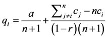 (10)
(10)
For our model, we assume that any firms stay in as far as the after-tax profit is greater than or equal to zero. With a process of a continuously increasing tax rate r, we assume that firms exits one by one. Let n(r) be the number of firms remained in business for a given r.
In the first stage, government chooses a tax rate, r, to maximize the total amount of tax revenue received, T:
 (11)
(11)
Notice that there exists a supreme for all feasible r, noted by rsup. It is the largest tax rate government could impose due to the limited fisheries stock. That is to say, any r high than rsup is not feasible.
The following method can be used as a good approach for finding an optimal r.
Lemma 1: Assume that a group S of existing firms can survive in the industry under a tax rate r (i.e. each has a nonnegative equilibrium profit) when no entry occurs, then when the tax rate is reduced to , these same group of firms can also survive.
Proof: We only need to show that, under the smaller tax rate, the new equilibrium profit for each firm increases.
Originally, the profit function for firm i is
 (12)
(12)
Substitute Equations (9) and (10) into Equation (12) and simplify:
 (13)
(13)
where , approximately equals ci.
At the critical point that firm i could survive, its profit equals to zero. Set Equation (13) equals to zero, we will get two solutions of r. In this case, we choose the smaller r because beyond this r firm i has already decided to quit the industry and the larger r is not feasible.
Take first-order derivative of Equation (13), we have:
 (14)
(14)
Equivalently:
 (15)
(15)
In this function, a denotes the maximum price determined by supply-demand mechanism and b is approximately equals to firm i’s marginal cost. Since firm i can survive at given r, its unit after-tax revenue (1 − r)a should be able to at least cover its marginal cost, b, and fixed cost per unit. Explicitly, (1 − r)a − b > 0 Thus  at r. In addition, from Equation (14) we know that when r decreases,
  also decreases. Therefore the derivative is negative for a given n on
 . By First Derivative Test,
  is decreasing on
 . Therefore, under the smaller tax rate,
  , the new equilibrium profit for each firm will be larger. To be exact, the same group of firms will remain survivable.
Let N be the number of all potential firms in fishery industry. Now let us consider all possible nonempty subset of the set of N firms. There are 2N − 1 of these subsets.
Definition: A subset S of firms is said to be coexistible if there exists a tax rate r ³ 0 under which each member in S earns a nonnegative profit and no entry will occur in the industry.
Now let us discuss the situations for coexistable subsets. Obviously the number of coexistible subsets of N is finite.
Lemma 2: For any coexistiblesubset S of firms, there must exist a maximal tax rate  such that under this tax rate S remains coexistible and at least one member in S has 0 equilibrium profit.
Proof: Because S is coexistible, there is a tax rate  under which each member in S earns nonnegative profit and no entry occurs in the industry. When the tax rate increases, by Lemma 1 no entry can occur, and at the same time the profit of each of the existing firm is reduced gradually. Note that each existing firm’s profit depends on r continuously, and as a result the smallest profit among them also continuously depends on r. The smallest profit is negative when r is increased to 1, by continuity there must exist some tax rate
  making this smallest profit exactly equal to 0.
Lemma 3: For any coexistible subset S of firms, either there exist some  such that entry into the industry will start to occur under this tax rate, or entry never occurs even the tax rate is reduced to 0.
Proof: The argument is trivial.
Let S be a coexistible subset of firms. Now we consider two different cases in Lemma 3.
Case 1: Suppose entry will occur when tax rate is reduced to rl(S).
The tax revenue T(S,r) for the government from these firms is continuously dependent on r in the interval on . In this interval, there is a least upper bound on government revenue. If it can be attained at some r-value
  within the half open interval, we will denote it
 ; if it is cannot attained within this interval, we define:

Note that  cannot be precisely achieved, but can be approximately achieved as r is reduced to sufficiently closed to but not equal to rl(S).
Case 2: entry will never occur When r varies from 0 to rh(S), the firms in S are always coexistible. Again we use .
.
Denote  to be either
  or
or . As there are at most 2N − 1 coexistible subsets, which is finite,
  has finite elements. Therefore, a maximum value among all the elements TM exists as either a maximum value achievable or a supremum.
To sum up we have Proposition 1: For each subset S of coexistible firms, let  be
be  or rl(S), dependent on whether or not the maximum of T(S) can be achieved within
 . Let
. Let  to be either
  or
or . Let
. Let . Then TM is either the maximum revenue achievable, or is the least upper bound.
4. Numerical Examples
To better illustrate the optimization process on government’s decisions, we give a simple example with all firms to be identical.
Suppose there are 5 potential firms in total in the industry, i.e. N = 5.
We randomly assign the values for parameters as follows:

As all firms are identical, all subsets of n firms, denoted by Sn, are exactly the same combination as long as nis fixed. We can simplify Equation (13) into
 (16)
(16)
Substitute the values into above equation:
 (17)
(17)
when r = 0, n = 5, we get ; i.e. the subset consisting all 5 firms is non-coexistible.
When r = 0, n = 4, we get ; i.e. the subset consisting 4 firms is non-coexistible.
When r = 0, n = 3, we get ; i.e. the subset consisting 3 or less firms are coexistible For subset S3 consist of 3 firms operating in the industry, to find
 , we set
  for Equation (17). Solving the equation gives us
 . When r decreases from 8.35% to 0, no entry will occur.
Government’s Revenue Function is:
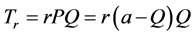 (18)
(18)
Substitute Equation (9) into Equation (18):
 (19)
(19)
Take the first-order derivative of Equation (19):
 (20)
(20)
Take the second-order derivative of Equation (19):
 (21)
(21)
By first-order derivative test,  is increasing for
  . Thus
 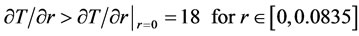 . Therefore T is an increasing function on
 . So we have
 .
.
We continue to solve the cases with subset S2 and S1 by similar methods and the results are shown in Table 1:
We plot T(Sn) against r for n = 1, 2 and 3, as shown in Figure 2.
The result shows that government can achieve the maximum revenue of 6.426 by imposing a revenue tax at the rate of 60.23% and when only one firm remaining in the industry.
5. Social Welfare Perspective
The total profit earned by the firms can be obtained by summing Equation (12) across the n existing firms, which is , where Q is the total harvest of all existing firms. Then the government’s revenue is
 . Define W as the net return from the entire fishery industry that is the summation of total profit from all the firms and the
government’s revenue, i.e.:
 (22)
(22)
Instead of achieving maximum revenue, government can also set tax rate r targeting to maximizing social welfare. The process of determining this r can follow the same method of finding the tax revenue maximization tax rate.
For each S of coexistible firms, consider welfare W(r) when r varies in . Either the maximum
  is attained within the interval at some
 , or the supremum
  is achieved as r tends to rl(S) from the right. Very much similar to the arguments for Proposition 1, we have Proposition 2: For each subset S of coexistible firms, let
  be
be  or
or , dependent on whether or not the maximum social welfare of W(S)can be achieved within
 . Let
. Let  to be either
  or
or . Let
. Let . Then WM is either the maximum social welfare achievable, or is the least upper bound.
In the example of identical firms above, substitute Equations (9) and (10) into Equation (22), we get the welfare function when all firms are identical:
 (23)
(23)
Plot W(Sn) against r for n = 1, 2 and 3.
Figure 3 shows that when government imposes a tax rate larger than but extremely close to rl(S3) = 37.98%, the social welfare can be ultimately close the maximum value. Yet this maximum value can never be exactly achieved. However, this preferred tax rate is clearly different with the tax rate that achieving TM, which is 53.18%.