Assessing the Economic Viability of France’s Pension Reforms Using AJ-LF Models

Anton Samokish, Georgii Kiselev, Ivan Minyaev, Kuzma Meleshin, Platon Ustinov, Ruslan Kerimov

Higher School of Economics, National Research University, Moscow, Russia.

DOI: 10.4236/tel.[phone]                

Abstract

The article is dedicated to the analysis of the Pension reform of 2023 in France. At the time of April 2023 this topic was hotly debated; many politicians, sociologists, economists, and common citizens expressed their opinions about Emmanuel Macron’s politics. The article examines the underlying reasons, background, and public response to the reform, as well as its immediate and long-term effects, through an unbiased investigation by developing a macroeconomic model for goods and labor markets. But what makes the study unique in its essence is a non-standard usage of game theory techniques: dominant and dominating strategies, Nash equilibrium in pure strategies. This approach provides readers with a unique and unconventional perspective on the situation, enabling them to gain insight into the motivations behind the actions of various stakeholders and improve their overall understanding of the consequences following the reform. At the end of the work authors provide a critical assessment of President Macron’s actions and answers to the most intriguing questions: “Was the introduced reform inevitable?”; “Perhaps it would be best to repeal the legislation and halt everything right here and now?” “Should Mr. President and the Government take public opinion into account, or it would be better to purely trust the view of professionals and proceed with the current political vector?”

Keywords

Pension Reform, France, Labor Market, Game Theory, Trade Unions

1. History of Pension Reforms in France

France is a country of ongoing reforms. At the beginning of 2023, a new pension reform was one of the most hotly debated topics in the world. “Protests and strikes in France in 2023 over pension reforms were striking evidence of the French people’s resolve to protect their social benefits and workers’ rights. While the administration contended that the modifications were required for the long-term viability of the pension system, the public saw them as unfair and skewed towards the rich.” (Bhattacharya, 2023; Bissuel, 2023; Hummel, 2023; Martin, 2023) . The situation is indeed curious, and we are going to study it in detail in this research. Nonetheless, before we begin, it is essential to provide a brief overview of the economic situation of past pension reforms in France.

1.1. History of Reforming the Pension System

Since Socialist President François Mitterrand lowered the retirement age from 65 to 60 years in 1982, the French government has been grappling with the challenge of adapting the pension system to account for the significant rise in life expectancy and the growing number of pensioners. Despite several attempts at reform, trade unions and the public consistently opposed them. This was the case when Alain Juppe’s government attempted to make changes in 1995 under Jacques Chirac’s leadership, but their efforts failed due to widespread strikes that lasted for several months, leading to the resignation of Juppe.

During Nicolas Sarkozy’s presidency in 2010, a pension reform was implemented which increased the retirement age from 60 to 62 years. Later, Francois Hollande, who succeeded Sarkozy, was able to partially reverse the unpopular reform by decreasing the retirement age by two years for citizens who began working at 18 - 19 years old.

1.2. The Reform of Emmanuel Macron

President Emmanuel Macron announced his plans for pension reform after he was elected in 2017, however, he had to postpone his plans due to the coronavirus pandemic. January 10, 2023, Prime Minister Elisabeth Born presented the statements on the pension reform. The main ones were an increase in the minimum retirement age up to 64 years and the abolishment of special pension regimes in various industries for new workers. The increase in retirement age is planned to be gradual by 3 months every year until 2030.

On March 16, 2023, the upper house of parliament approved the final version of the document, and Prime Minister Bourne took responsibility for its approval by invoking Section 3 of Article 49 of the constitution, fearing it would not be approved by the National Assembly. On March 22, opposition deputies submitted requests to assess the constitutionality of certain provisions of the bill, which usually takes about a month for consideration, with up to eight days for an accelerated procedure. On April 17, 2023, Mr. Macron announced that the reform would come into force in the autumn of 2023.

1.3. Background and Causes of Pension Reform

The diagram in Figure 1 illustrates the demographic situation in France as of the

Retrieved April 26, 2023 from: https://www.populationpyramid.net/france/2023/.

Figure 1. Population distribution in France.

beginning of 2023. Ideally, the bar size should decrease with the rise in the age group, then there is enough money from the working population’s pension contributions to pay benefits to pensioners. However, we see a decline in the age range of 20 - 44 and a decrease in current birth rates. This leads to an imbalance between the working-age population and pensioners, which places a heavy burden on the budget.

French authorities predict that the number of pensioners will only increase from 17 million people to 20 million in 2030, causing a pension budget deficit of up to 20 billion euros. The pension reform was required, but it was delayed by previous presidents due to its unpopularity. The introduction of the reform crucially reduces the chances of re-election. Emmanuel Macron was in his second presidential term, which is the maximum allowed. So, his potential losses from the unpopular reform were much lower. It was time to act.

Now we can move on directly to the analysis of the current situation. However, before we start, we should give a brief theoretical overview of the economic models that we are going to use in our study.

2. AD-AS Model

Our study is based on macroeconomic models. The first we are going to introduce is an AD-AS:

The AD-AS model is a way of illustrating national income determination and changes in inflation. It can be used to illustrate phases of the business cycle and how different events can lead to changes in two key macroeconomic indicators: real GDP and inflation (Barro, 1994) .

2.1. Structure of the Model

· Two axes: a vertical one labeled “Inflation” and a horizontal axis labeled “real GDP.”

· A downward-sloping aggregate demand curve labeled “AD.”

· An upward-sloping short-run aggregate supply curve labeled “SRAS.”

· A vertical long-run aggregate supply curve labeled “LRAS.” It represents the natural level of output.

2.2. Assumptions of the Model

1) Flexible prices and wages, signifying that inflation plays a significant role.

2) Nominal and real interest rates are different.

3) Fixed nominal wage growth rate.

4) Wage expectations reflect inflationary expectations.

5) Existence of trade unions with high bargaining power.

6) Flexible inflation targeting is the monetary policy utilized.

7) The government adheres to the balanced budget rule.

2.3. Derivations

2.3.1. Aggregate Demand (AD)

$Y=AE\left(Y,r\right)=A{E}_0-br+mpe\ast Y$

When the Central bank pursues flexible inflation targeting, the monetary policy (MP) rule is:

$r=r^{*}+a\left(\pi -{\pi }^{*}\right)$

From national income identity:

$Y=AE\left(Y,r\right)=A{E}_0-b\left(r^{*}+\alpha \left(\pi -{\pi }^{*}\right)\right)+mpe\ast Y$

$Y=AE\left(Y,r\right)=A{E}_0-b{r}^{*}-b\alpha \pi +b\alpha {\pi }^{*}+mpe\ast Y$

$b{r}^{*}+b\alpha \pi -b\alpha {\pi }^{*}=A{E}_0-Y\ast \left(1-mpe\right)|\ast \frac{1}{b}$

$r^{*}+\alpha \pi -\alpha {\pi }^{*}=\frac{A{E}_0}{b}–\frac{1-mpe}{b}\ast Y$

$\alpha \pi =\alpha {\pi }^{*}-r^{*}+\frac{A{E}_0}{b}–\frac{1-mpe}{b}\ast Y|\ast \frac{1}{\alpha }$

Thus, AD schedule becomes:

$\pi ={\pi }^{*}-\frac{r^{*}}{\alpha }+\frac{A{E}_0}{\alpha b}–\frac{1-mpe}{\alpha b}\ast Y$

2.3.2. Short-Run Aggregate Supply (SAS)

$\pi ={\pi }^e+\lambda \ast \left(Y-Y_N\right)$

2.3.3. Long-Run Aggregate Supply (LRAS)

$Y=Y_N$

2.3.4. Interpretation of Variables

· Y - real output

· $Y_N$ - full employment level of output

· $A{E}_0$ - autonomous expenditure

· mpe - the marginal propensity to expend

· b - investment demand sensitivity to interest rate

· r - real interest rate

· $r^{*}$ - targeted real interest rate

· $\alpha$ - aggressiveness of Central Bank to eliminate the inflation gap

· $\pi$ - inflation rate

· ${\pi }^{*}$ - targeted inflation rate

· ${\pi }^e$ - expected inflation rate

· $\lambda$ - positive constant: an indicator of how much inflation responds to changes in output.

The model is effective in examining the impacts of macroeconomic disturbances on overall income and inflation levels. In the case of the pension reform, due to the raised retirement age, some individuals who would have retired earlier will now continue working until they reach the updated retirement age. Hence, the total number of working people will be higher which will lead to a higher level of potential output ( $Y_N\uparrow$ from $Y_N^0$ to $Y_N^1$ ) as more people will join the labor force. All else being equal, the increased labor force will give the economy an opportunity to produce more output. As a result, aggregate supply will increase in the long run perspective which will be indicated by the rightwards of the SAS and LRAS schedules. This process is illustrated in Figure 2 by the transition from the initial equilibrium (0) to the subsequent (1).

3. Application of AJ-LF-L^D Model

Another model applied in our research is the Labor market AJ-LF-L^D model which is a way of illustrating the situation in the labor market including changes in unemployment and real wages.

3.1. Model Structure

· Two axes: a vertical one labeled “Real wage” and a horizontal axis labeled

Figure 2. AD-AS.

“Quantity of Labor”.

· A downward-sloping labor demand curve labeled “L^D”

· An upward-sloping “AJ” curve shows the number of people in the labor force willing to accept job offers at any level of real wage.

· An upward-sloping “LF” curve illustrating the size of labor force.

· AJ is to the left of LF because some members of the labor force are between jobs, and others are waiting for better offers.

· Trade unions use their power to force firms to pay higher wages.

3.2. Assumptions of the Model

In addition to the assumptions for the AD-AS model, the model requires that labor and capital are complements as inputs.

3.3. Formulas

$Y=F\left(K,L\right)$ $LF=\phi +\xi w$ $AJ=\left(\xi +\psi \right)w$ $L^D=MPL+\zeta$

Interpretation of Variables

· L - number of workers (quantity of labor)

· W - nominal wage

· P - price level

· $w=\frac{W}{P}$ - real wage (or just wage in further analysis)

· F(K, L)- production function with complementary inputs

· AJ(w) - the number of workers in the labor force willing to accept jobs at a given real wage. We consider only the upward-sloping segment of AJ curve.

· LF - function indicating the number of people in the labor force at a given real wage.

· φ - parameter, indicating the wage insensitive number of people in the labor force, i.e. number of unemployed in the labor force when w = 0

· ξ - parameter, indicating the number of people joining labor force and willing to accept job at new wage level when real wage increase by 1 basis unit

· ψ - parameter, indicating the number of workers by which the natural rate of unemployment (NRU) increases, when wage level decreases by 1 basis unit.

· L^D - labor demand function

· ζ(K) - parameter, indicating the complementary nature of inputs. It shows that the higher is the stock of capital, the more labor is demanded to operate the capital.

We will consider different cases based on the decisions of two players: the government and trade unions. The government must determine if they will force the pension reform or reverse it, while trade unions face the decision of either agree with the reform or will fight with it. Our model will analyze all these cases and show the corresponding outcomes in relation to the equilibrium labor quantity and real wage.

4. Model Extension

The standard AJ-LF-L^D and AD-AS models described above cannot provide a complete breakdown of the pension reform shocks. Consequently, the model should be modified and extended for proper research. It must consider the pension reform implementation by the government and the possible reaction of the trade unions to this reform.

So, we modified the model with elements of game theory to show that in this situation government does not conduct decisions unilaterally-it should account for trade unions decisions also.

4.1. Assumptions

1) There are two “players” in the model: the government and trade unions that make their decisions simultaneously.

2) The government can conduct one of two actions: force the reform to impose or revert the initial decision and cancel the reform introduction.

3) Trade unions can conduct one of two actions: try to fight with a reform by protesting and staking or agreeing with the reform and not interfering in internal politics.

4) The government sticks to the balanced budget rule that is consistent with empirical facts in the long run.

5) Trade unions are very powerful, consist of many workers and may significantly influence the labor market equilibrium. That assumption reflects the nature of trade unions in France, where their influence is substantial.

4.2. The Model Basis

To begin with, an extended model acts as a framework for understanding the determinants of wages, employment, and labor market outcomes. The model considers labor demand and the institutional structures that influence the bargaining power of workers and firms. In this section, the model will be set up to explore the key drivers of employment and wage outcomes, as well as the potential impact of policy interventions. The aim is to contribute to a deeper understanding of the complex dynamics that shape the labor market and inform evidence-based policy decisions.

To establish a model (Figure 3), we first defined the variables involved and developed a theoretical framework to guide our approach. The AJ and LF functions were described above, in the model they will be given by functions:

$LF=\phi +\xi w$

$AJ=\left(\xi +\psi \right)\ast w$

Labor demand is given by:

$L^D=MPL+\zeta$ , where MPL is a linear function.

In the initial allocation (0) trade unions have already used their power to negotiate better wages, benefits, and working conditions for their members:

Firstly, let’s focus on the cases when trade unions decide not to fight against the reform and, therefore, not engage in industrial action, such as strikes, to put pressure on employers and government to meet their demands. Secondly, we will consider cases, when trade unions decide to fight with the reform to prevent its implementation.

4.3. The Game

4.3.1. Case 1: “Effects of Government’s Decision to Force the Reform”

In this case, the government decides to force the reform, while trade unions apply no pressure on the officials and just agree with the conducted policy. Then, due to pension reform implemented, number of people in labor force increases irrespective to wage that means that φ increases. However, not all “new”

Figure 3. AJ-LF.

non-pensioners will be willing to work at any wage rate and not all will even join the labor force immediately which implies the increase in ξ. Some of them will not find the loss in pension transfers so critical, for instance. Overall, compared to the initial allocation, the AJ curve will rotate to the right around the origin and LF schedule will shift and rotate to the right. In the new equilibrium, trade unions remain powerful causing increased unemployment but no change in labor employed.

Now, let’s turn to the AD-AS diagram. When the government forces the reform, it reduces the number of transfers it should pay to its citizens NT↑, consequently, the budget surplus occurs (BD < 0) (Figure 4).

“Increasing the retirement age reduces retirement benefit payments and raises income and payroll tax revenues, thus reducing the government’s financial burden” (Staubli & Zweimüller, 2013) . As the government sticks to the balanced budget policy, it will increase its government purchases G↑. Therefore, due to multiplier effect (∆G + c₁∆NT > 0) there occurs a favorable shock of aggregate demand and AD↑. Increased level of government purchases implies more investment in public infrastructure that increases the stock of capital in economy K↑. Higher stock of capital leads to a rise in labor demand due to the complement nature of inputs that is indicated by the rise in parameter ζ↑. (Figure 5)

This would result in un rightward shift of the L^D schedule. (Firms could not hire more labor by moving down their existing labor demand due to wages set up by powerful trade unions).

So, more labor will be hired that results in higher output and transition from point (0) to point (1).

In the long run, due to a change in natural rate of unemployment and higher level of employment, the LRAS and SRAS schedules will shift to the result in an equilibrium in point (2).

Figure 4. AJ-LF in Case 1.

Figure 5. AD-AS in Case 1.

4.3.2. Case 2: “Effects of Government’s Decision to Reverse the Reform, While Trade Unions Agree with It”

In this case despite the trade unions deciding to agree with the reform for a certain reason government reverts it back. Therefore, in this case, no change will occur in either labor or goods market, so the economy will stay at its initial level at point (0). This scenario is intended to depict the potential for the government to unilaterally reverse the reform, even if trade unions choose not to directly oppose it.

4.3.3. Case 3: “Effects of Trade Unions Decision to Fight with the Reform”

When trade unions decide to fight, they start protesting, stacking and stop working. Hence, the Labor Force remains intact, while there occurs a proportion of people that will not work for any wage offered. Then, new AJ function can be given by:

$AJ=\min \left\{\left(\xi +\psi \right)\ast w;\phi +\xi w-\theta \right\}$

where, θ - the number of people in LF force not willing to accept job at any wage. As trade unions are very powerful, a substantial proportion of the population belongs to them. Hence when trade unions protest, number of protestants θ is high. Therefore, high θ not allow the economy even to reach the initial output level. (Figure 6)

1) In AJ-LF diagram: φ↑, ξ↑ that lead to rotation of both kinked parts of AJ schedule and rightward shift and rotation of the LF curve.

Figure 6. AJ Transformation.

Also, G↑ lead to higher capital stock K↑ => ζ↑ due to the complementary nature of inputs => L^D ↑ and shifts rightwards.

2) In AD-AS diagram: NT↑ => BD < 0 => G↑ as government sticks to balanced budget => AD↑ due to multiplier effect. In long run: LRAS, SRAS shift rightwards as the new potential level of output is higher because of higher potential level of employment. (For more detailed explanation, examine the section about effects of pension reform in case 1).

As the influence of labor unions in the economy is so high the resulting SR labor market equilibrium will occur at lower number of labors employed at even higher wages than before. Consequently, the cost of factors of production rises that lead to the leftward shift of the SAS schedule. So, in SR equilibrium (2) the effect on output is ambiguous while inflation will rise (SRAS may even further upwards). Nevertheless, in the long run, when trade unions workers come back to their working places, the SAS schedule will move to its initial position. So, in a new equilibrium (3) the level output will be higher than before the shock (Figure 7):

4.3.4. Case 4: “Effects of Government’s Decision to Reverse the Reform, while Trade Unions Fight with It”

In this case (Figure 8) trade unions fight with the proposed pension reform and the government, influenced by their demonstrations, reverses its initial decision and cancels the reform. In this case the government pension reform will not influence the economy as the shifts in AJ, LF, AD schedules will be reverted to their initial position. In the SR when workers of trade unions are stacking and demonstrating, new labor market equilibrium occurs at higher wages and lower labor employed. Therefore, the cost of factors of production rises leading to un leftward shift of the SAS schedule. So, in SR equilibrium the output will be lower

Figure 7. AJ-LF in Case 3.

Figure 8. AD-AS in Case 3.

Figure 9. AJ-LF in Case 4.

Figure 10. AD-AS in Case 4.

than initial, while inflation will be higher than the pre-shock level (1). In the long run members of trade unions will come back to work and the economy will return to its pre-reform equilibrium (0):

4.3.5. Comparison of Outcomes and Bimatrix Construction

Consider the 2 × 2 bimatrix given below where payoffs of players in case “i” are given by (g_i, t_i). To determine the parameters of the bimatrix, analysis of the outcomes from both government and trade unions side is performed:

From this analysis we can deduce the following inequalities:

1) $g_1>g_3>g_2=0>g_4$

2) $t_2=0>t_4>t_1>t_3$

Based on these inequalities we can form a resulting bimatrix:

By analyzing the game, it can be outlined that government has a dominant strategy: to force the reform. The best response to this strategy by the trade unions is to agree with the initiated reform. Consequently, the Nash Equilibrium (NE) in pure strategies in this game is (Force, Agree). Therefore, the government is able to end up in the most beneficial outcome after the reform implementation. So, Emmanuel Macron’s decision to enforce the reform is now supported by the macroeconomic model. Overall, the model shows that the reform will result in the rise in the employment and hence the rise in aggregate output. However, the impact on unemployment remains unclear, as the number of individuals joining the labor force and remain unemployed might be significantly greater than those who joined the labor force and were able to secure employment. The observed findings are consistent with the research conducted by Geyer et.al. (Geyer et al., 2021) that covers the consequences of a similar reform in Germany: “We showed that the reform had the expected positive effects on employment and, to a lesser extent, unemployment…” (Geyer et al., 2021) .

5. Summary & Conclusions

To sum up, through our research, we determined that recent pension reform in France was almost inevitable from the macroeconomic perspective. Increase in demographic imbalance throughout past decades has been gradually leading to a huge pension deficit, and an increase in the pension age is one of the most efficient methods to cure it. Obviously, such reform has caused massive unrest over the entire country, people created unions and started to protest the policy that forces them to work more.

With the implementation of AD-AS and AJ-LF-L^D models and analyzing all possible outcomes using the game theory, we concluded that the most optimal and socially beneficial outcome will occur in case if people stop arguing and accept the reform. In the long run it will help to improve the pension deficit and will lead to an increase in the overall performance of the economy. Also, if unions persist in their demonstrations, it could further deteriorate the situation and potentially make it irreversible.

However, at the beginning of 2023, the public was not planning to stop protesting, even increasing the degree of heat. From day to day, more and more people took part in demonstrations, causing entire sectors of the economy to stall. The situation has developed according to the most negative scenario that potentially has many adverse consequences that will pull French economy back. Nonetheless, we believe that the choice to enforce the reform made by Emmanuel Macron and his administration is the sole appropriate course of action, given that its benefits significantly outweigh its disadvantages.

The model used and applied in the analysis has several limitations. Firstly, it considers the simultaneous game only of two players with two distinct pure strategies, and just several variables reflecting the labor market equilibrium, while there can be many more influential players and factors. In further research of pension reform consequences, the introduction of new players and a wider range of strategies including mixed ones should be considered. Secondly, the model proposed does not account for the very long run effects due to assumptions of the AD-AS and AJ-LF models. Nevertheless, in further studies, this can be extended by applying the Solow model to the same shock. Alternatively, one can apply the infinite games approach to the sample game set up above to examine the effects of the reform in the very long run.

Appendix

A1. Estimation of Parameters of AJ-LF Model

A1.1. LF Function

As we know, LF function is:

$LF=\phi +\xi w$

To estimate parameters φ and ξ we collected data about the France’s labor force (in millions) and average annual wage (in current ? for the period from 2000 to 2021. We constructed a regression model based on this data, assuming φ to be α (alpha) and ξ to β (beta).

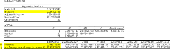
We obtained the following results:

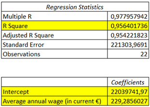
(Full data and regression tables can be seen in appendix 7.2)

$R^2\approx 0.956$ means that 95.6% of variability in Labor Force can be explained by the regression model i.e., there’s a very strong correlation between labor force and average annual wage.

· Intercept = 22,039,741.97 implies that

$\phi =22039741.97$

· Average annual wage (in current ? ≈ 229.29 implies that:

$\xi =229.29$

Thus, we obtain the LF function equal to:

$LF=22039741.97+229.29\ast w$

A1.2. AJ Function

We have already estimated parameters φ and ξ. Currently, an unknown parameter for us is only ψ.

As we know, ψ – number of workers by which NRU increase, when wage level decreases by 1 basis unit.

AJ and LF functions are:

$LF=\phi +\xi w$

$AJ=\left(\xi +\psi \right)w$

$LF-AJ=NRU=\phi +\xi w-\left(\xi +\psi \right)w$

$NRU=\phi +\xi w-\xi w-\psi w$

$NRU=\phi -\psi w$

Thus, we obtained $NRU-\phi =-\psi w$

For the regression model we assumed $-\psi =\beta$ and, as a result, estimated:

$NRU-\phi =\beta w$

· Parameter φ was already estimated in LF function.

$\phi =22039741.97$

· NRU was observed in number of people by gathering Frances’s natural rate of unemployment rate for the period from 2000 to 2021 and multiplying it by the number of people in labor force (was already recognized in calculating parameters of LF function) in each corresponding year.

· Average annual wage (in current ? w was also already observed in calculating parameters of LF function.

By constructing the regression model, we obtained following results:

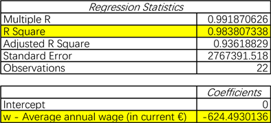
(Full data and regression tables can be seen in appendix 7.3)

$R^2\approx 0.984$ means that 98.4% of variability in (NRU-φ) can be explained by the regression model i.e., there’s a very strong correlation between (NRU-φ) and βw.

Average annual wage (in current ? ≈−624.49 implies that

$\beta =-624.49$

As $-\psi =\beta$ , it can be derived that $-\psi =-624.49\Rightarrow \psi =624.49$

Thus, $NRU=22039741.97-624.49w$

Consequently, AJ function becomes:

$AJ=\left(229.29+624.49\right)w$

$AJ=853.78\ast w$

A2. Data for Estimation of Parameters of LF Function

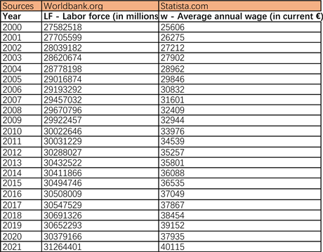
A3. Data for Estimation of Parameters of AJ Function

Conflicts of Interest

The authors declare no conflicts of interest regarding the publication of this paper.

References

[1]	Barro, R. (1994). The Aggregate-Supply/Aggregate-Demand Model. https://www.jstor.org/stable/40325537
[2]	Bhattacharya, S. (2023). Nationwide Protest in France in 2023 Against Proposed Pension Reform. International Journal of Multidisciplinary Research and Publications, 6, 72-75. http://ijmrap.com/wp-content/uploads/2023/11/IJMRAP-V6N5P124Y23.pdf
[3]	Bissuel, B. (2023). Pension Reform: What France’s Largest Labor Union Has to Say about It. https://www.lemonde.fr/en/france/article/2023/01/11/pensions-france-s-main- labor-union-s-take-on-successive-reforms_6011204_7.html
[4]	Geyer, J., Haan, P., Lorenz S., Zwick, T., & Bruns, M. (2021). Role of Labor Demand in the Labor Market Effects of a Pension Reform. Industrial Relations, 61, 152-192. https://doi.org/10.1111/irel.12293
[5]	Hummel, T. (2023). French Unions to Keep up Pensions Protest after Talks with PM Fail. https://www.reuters.com/world/europe/frances-labour-union-leaders-say-talks-with-pm-yielded-no-results-2023-04-05/
[6]	Martin, E. (2023). Pension Reform in France: Diagnosis of a Crisis. https://www.gisreportsonline.com/r/france-pension-reform/
[7]	Staubli, S., & Zweimüller, J. (2013). Does Raising the Early Retirement Age Increase Employment of Older Workers? Journal of Public Economics, 108, 17-32. https://doi.org/10.1016/j.jpubeco.2013.09.003