Adapted Metrics for a Modified Coulomb/Newton’s Potential

Lucian M. Ionescu^1*, Cristina-Liliana Pripoae², Gabriel Pripoae³

¹Department of Mathematics, Illinois State University, Normal, IL, USA.
²Department of Applied Mathematics, The Bucharest University of Economic Studies, Bucharest, Romania.
³Faculty of Mathematics and Computer Science, University of Bucharest, Bucharest, Romania.

DOI: 10.4236/jhepgc.2023.94090                

Abstract

Modified Theories of Gravity include spin dependence in General Relativity, to account for additional sources of gravity instead of dark matter/energy approach. The spin-spin interaction is already included in the effective nuclear force potential, and theoretical considerations and experimental evidence hint to the hypothesis that Gravity originates from such an interaction, under an averaging process over spin directions. This invites to continue the line of theory initiated by Einstein and Cartan, based on tetrads and spin effects modeled by connections with torsion. As a first step in this direction, the article considers a new modified Coulomb/Newton Law accounting for the spin-spin interaction. The physical potential is geometrized through specific affine connections and specific semi-Riemannian metrics, canonically associated to it, acting on a manifold or at the level of its tangent bundle. Freely falling particles in these “toy Universes” are determined, showing an interesting behavior and unexpected patterns.

Keywords

Modified Gravity Theory, Spin, Coulomb’s Law, Newton’s Law, Modified Coulomb’s Law, Nuclear Force, Adapted Connection, Adapted Metric

1. Introduction

Our physical take on the Universe is based on two “Standard Models”: Cosmology, based on General Relativity, including Big-Bang Theory (inflation, matter genesis, large scale structures etc.) provides a macro-Cosmos, large scale model in Space and Time for Matter and its Dynamics/Structure; on the other hand, The Standard Model of Elementary Particle Physics (EPP SM) studies the micro-Cosmos, classifying the elementary constituents and their interactions, in terms of the so called fundamental forces.

A preliminary justification of our project, in the above context, is followed by a detailed explanation of the motivation for this approach, and how it fits in the historical development of the subject (Newton, Einstein, Klein, Cartan etc.), with emphasis on the minimal solution” (extension of Coulomb Law) and mathematical framework adequate for Cosmology (Einstein-Cartan Moving Frame Theory).

1.1. How This Project Started

This is a project part of a larger research program aiming to several levels of unification in Sciences, especially in Physics¹.

1.1.1. Separation in Physics

A considerable effort in Cosmology is invested in upgrading GR in order to account for large scale discrepancies in its predictions vs. more and more accurate and extensive data. On the other hand, there is a need to go beyond the SM, to address known limitations of the SM. One major (overlooked) such limitation resulted from the EPP community totally ignoring Gravity, still considered a fourth fundamental interaction, because it is too weak to be measured and studied in the Lab (with particle accelerators or low temperature physics not honed for such a study; and because of conflicts of interest...).

The need to bridge the gap between the two SM-s is obvious, to avoid Cosmology having to solve its own problems (e.g. dark matter/energy etc.) which belong naturally to the other camp.

1.1.2. A Bit of History

The historical trend, quantization of Classical Physics, led to the culture that General Relativity has to be quantized, towards a quantum theory of Space-Time-Matter-Gravity theory, called Quantum Gravity.

But by now there is a lot of progress in other areas (solid state physics, quantum Hall effect, superconductibility, Quantum Computing—software and hardware etc.) inviting to reconsider the approach, and attack the Graal of Physics, from another direction: unify Gravity and Electromagnetism, as a byproduct of unifying ElectroWeak Theory and Quantum Chromodynamics. The key point is to understand that positive charges are not pointwise, and that both the neutron and proton have an electric charges quantum structure which might be responsible for the Gravitational Force as a correction to the Electric Force.

1.1.3. A Possible Breakthrough

This avenue of research and development in EPP beyond the SM has a long history [2] [3] [4] [5] [6] , targeting also Gravity, at the level of experiment and theory, both peer-reviewed (e.g. F. Alzofon, Podkletnov, Li Nang [7] ) and prospective. The facts established so far without a doubt include the following: rotation, magnetic fields and superconductivity, together with Dynamic Nuclear Orientation based on electron orbital-nuclear spin coupling, exhibit force effects and phenomena which cannot be explained by EM, affecting the weight of the object involved.

Note the parallel: not only GR based dynamics cannot explain all “Cosmological Data, but also SM based phenomenology cannot explain all Lab data”... Maybe there is a common reason?

1.1.4. “Einstein Is Always Right”

While this is still a long road to follow, a line of research on the other “camp”, Cosmology, consists in developing the Einstein-Cartan Theory [8] (Moving Frame geometry) as a framework to accommodate an effective theory of spin-spin interaction in a mathematical framework based on connection geometry which includes a theory of spin!

This provides a common language with the gauge theory approach in the SM and prepares the formalism to accommodate quantum spin at EPP level².

1.1.5. The Journey of 1000 Miles

Our long-term plan of R&D (bridging the two SMs) was sketched in several preliminary articles [4] [9] [10] (not peer-reviewed), reaching the above conclusion, that an improved, gauge theory friendly mathematical framework including a spin-spin interaction is needed, as a continuation of the line of research initiated by Einstein (teleparallelism, tetrad approach) based on Cartan Moving Frame geometry. This will be a part of Alternative Theories to GR, a big tree with MOND [11] [12] and Scalar-Tensor-Vector Gravity [13] as branches, which both have entertained the use of Yukawa nuclear force potential to modify the Newton (Coulomb like) force law to account for the mentioned discrepancies.

1.2. Why Invest in It...or Just Come along with Us!

The advantages of our approach are: 1) We design a framework as an effective theory, independent on the “quantum details” corresponding to the nuclear distances and model for the baryon quark field; 2) It can model a gravitational charge both positive and negative, as proved by experiment: F. Alzofon [5] , reproduced by other R&D groups [7] [14] (see also Li Nang, Podklednov etc. [6] ) and predicted by theory (new advancements in the SM, based on a reinterpretation of the quark model [3] [2] ); 3) It is a continuation of Einstein’s work and extraordinary intuition of Cartan³; 4) The value of such a development is independent on the validation of the cited publication not peer-reviewed.

1.3. Motivation and Background

There exist extensive Cosmological data supporting that General Relativity (GR) does not accurately models Gravity and Space-Time-Matter Dynamics, according to the amount and distribution of mass and energy-momentum in the Universe that we account for [15] .

A modification of GR, as an alternative to introducing dark matter and energy, is called Modified Gravity Theory (MGT) [16] [17] [18] . In these theories, correction terms are introduced, of the same geometric nature as in GR, e.g. involving an additional R² term in the Einstein-Hilbert action, the square of the curvature tensor.

In a totally different direction, from Cosmology to Particle Physics, experimental physics demonstrated a connection between gravity, rotation and magnetic fields [5] [6] . This is expected if we take into account the quark structure of nucleons, with the three distinct fractional electric charges, of opposite signs, with their orientation given by spin, as in the Standard Model of EPP.

This (Theory and Experiment) suggests that gravity is of quantum origin (not to be confused with Quantum Gravity as a theory quantizing GR!), a correction to EM due to the internal structure of nucleons.

1.3.1. Gravity and Nuclear Spin Orientation

Indeed, several experiments consistently proved that gravity is nuclear spin orientation dependent [5] [7] [14] . The theoretical model and justification comes from analyzing the quark structure of nucleons, an essential part of the Standard Model of Elementary Particle Physics [19] . This is quite a recent line of research in the 2020s, and like a similar breakthrough (Quark flavors corresponding to Platonic symmetry groups: [2] [3] 1990s), are not yet developed at “textbook level”, to be included in the mentioned SM. Furthermore, the fact that Gravity is so weak is a deterent in EPP to be studied experimentally, and hence it is planely ignored completely (relying on GR as a “standard model” for Gravity).

This approach, of identifying Gravity with a correction of EM component of nuclear fields, is natural because: 1) There is extensive experimental evidence in the laboratory [6] ; 2) Gravity is systematically neglected in Elementary Particle Physics (Standard Model) and High Energy Physics; 3) The formal separation between the other three fundamental interactions within the Standard Model, or more accurately between the Electro-weak Theory and QCD prevents for the understanding of “fine structure” of nucleon interactions.

In this paper, we build a simple theoretical model by introducing a spin-spin interaction term, as a correction to the classical electric force, modeled by Coulomb’s Law, in the point-wise charge model. This is an effective way to account for the structure of a nucleon, including the structure of the electric, i.e. divergent, component, which is modeled as fractional charges of their quarks.

Below we included a schematic picture of the electron-proton scattering experiments in the 1960s that proved that the proton, hence the neutron also, has a complex structure, including its electric field [20] .

Further electron-deuteron scattering experiments in the 1970 [21] confirmed that neutrons too have a complex electric field, and are not electrically neutral! The mathematical fact that algebraic sum of the fractional charges of the neutron’s “partons” (generic term for internal parts), does not mean the neutron’s electric field is a linear superposition of pointwise isotropic (fractional) charges; hence if the quarks are not accurately modeled as pointwise charged (electric

and color) particles, then a tensorial/complex non-isotropic vector field modeled is needed; hence the idea of a minimal modification of Coulomb’s Law, to account for a directional contribution, spin related.

Comparing with the currently accepted theory, we found that Nuclear Physics already accounts for such a contribution to the effective potential of the Nuclear Force [22] , without reference to Gravity.

Remark 1.1. Note that some obvious immediate consequences ensue, by similarity with EM: polarization effects! In fact the two theories, EM and Gravity correction, have much more in common, since the magnetic field (direction) is essentially due to electron orbital “spin” (with a contribution from intrinsic spin) and, we claim Gravity is due to nucleon’s spin (and maybe a contribution from an analog of internal nuclear orbits).

1.3.2. Pointwise Charge vs. Baryon Field

Note that the Coulomb electric field is isotropic, i.e. SO(3) invariant, as demanded by modeling electric charges as pointwise.

In reality (experimental physics), the negative electric charge we denote by e⁻ is totally different, in structure, from the positive electric charge of the proton. Even the neutron, electrically neutral when modeled as a pointwise particle, has a non-trivial electric charge structure, consisting of two directions repelling as a −1/3e⁻ fractional electric charges, and one direction with an electric (divergent) field equivalent to a −1/3 fraction of the electron’s electric charge e⁻ [23] .

An early attempt to unify EM and quark model of EPP, based on a “stringy” version gauge theory, aiming to construct the electron, meson and baryon fields from a quantized magnetic flux was done by Jehle [24] [25] [26] [27] . Both the emergent magnetic flux and electric field of elementary particles (electron and baryon) were derived in a way which is compatible with the present approach and previous proposal of the first author [28] ⁴.

1.3.3. Nucleon Electric Field’s Complexity May “Hide” Gravity

We included these details to convince the reader that there is much more to understand regarding the electric field of the nucleons (and electrons), beyond the classical isotropic, Coulomb Law.

At present, the Standard Model “struggles” with other issues, and the above presented considerations are studied by various researchers and laboratories independently, not being “ready” to be incorporated into the SM.

In fact several other authors claim that the Standard Model already contains the necessary ingredients to model the new Theory of Gravity [28] (see also references within).

1.3.4. Preparing the Way

What is clear so far, is that a non-isotropic “Coulomb Law”, spin direction dependent needs to be studied and that such a model can explain the experimental evidence mentioned above.

At the same time, this is a “perfect fit” for developing Einstein-Cartan generalization of GR, which incorporates spin as a source of torsion.

Once the theory will be developed, starting with the evidence in the Lab, at micro-cosmic level that Gravity maybe of nuclear origin and its strength, spin direction dependent, one would have to derive the consequences. Then, one would have to compare the observational evidence involving rotating masses exhibiting EM fields; such “spin data” needs to be fed into the Einstein-Cartan Model including a spin-spin interaction term in the Lagrangian, conform with the proposed Modified Coulomb Law. Finally, the dynamics needs computed, and analyzed if the resulting dynamics explains the known observational data, explaining the discrepancies and deviations from GR predictions.

1.4. History

The pillars of Gravity theory are two, so far: Newton’s Theory and Einstein’s General Relativity.

1.4.1. Newton’s Gravity

Newton gave the first theory of gravity, within the framework of Classical Mechanics:

$F=ma\left(\text{Framework}\text{for}\text{Dynamics}\right)$

$F_G=G\frac{mM}{r^2}\left(\text{Constitutive}\text{Law}\text{of}\text{Gravity}\right)\mathrm{,}$

especially designed for the derivation of Kepler’s Laws. These were conjectured based on the observational data gather by Tycho Brahe. There are a few additional assumptions: central force and always attractive.

One can then separate a gravitational field intensity E_G, derived from a gravitational potential, from the force itself:

$\begin{array}{l}\text{Particle}\mathrm{<mo>\; :\; </mo>}{\stackrel{\to }{F}}_G=Gm{\stackrel{\to }{E}}_G\mathrm{,}\text{Field}\mathrm{<mo>\; :\; </mo>}{\stackrel{\to }{E}}_G=-grad\left(U\right)\mathrm{,}\\ \text{Potential}\mathrm{<mo>\; :\; </mo>}U\left(M\mathrm{<mo>\; ;\; </mo>}{\stackrel{\to }{r}}_P\right)=M\frac{1}{r}\mathrm{<mo>\; ;\; </mo>}r=\left|{\stackrel{\to }{r}}_P\right|\mathrm{.}\end{array}$ (1)

We assume the source of the field is an object of mass M at the origin of the coordinate system. (Here we use the traditional notation for the electric field intensity.)

This is typical of field-particle theory, where determining the dynamics of the probe in a field generated by a distribution of sources is the main direct problem. Note that the charge of the probe, which measures the response of the probe in a given field, decouples from the charge for the source, and the interaction strength is proportional to their product (reflects the superposition of individual contributions from the elementary particles constituting the two bodies, corresponding to a bipartite graph).

It turns out that Newton’s Law for gravity is a modification of the universal paradigm of static force fields, central and isotropic, embodied in Coulomb’s Law as a central piece of Electrostatics. These modifications (only positive charges and different sign in the force law) were needed to have gravitational force always attractive. A speculative analysis points towards the conclusion that Gravity is of quantum origin [29] .

1.4.2. Einstein’s General Relativity

General Relativity represents an unprecedented change of paradigm: 1) Model of the Universe as a whole, leading to Cosmological models, including a scientific theory of Genesis; 2) Its model for interactions, dedicated to Gravity, but later extended as in kaluza-Klein Theory, uses a deformation of the (space-time) metric, which anticipates the introduction of propagators in QFT.

Remark 1.2. Newton’s Law of Gravity solves Poisson equation as the fundamental solution (later Green’s function in Klein-Gordon equation etc.). The PDE-symbol of the Laplacian is the Euclidean metric. If one changes the metric Green function changes; the next paradigm is that of QFT, which specifies the Green function itself, as the propagator, in a background metric, usually euclidean.

This allows to encode dynamics as geometry: dynamic trajectories as (metric) geodesics. Later on the Gauge Theory paradigm advanced by using connections, i.e. using parallel transport rather than the metric’s Levi-Civita connection. 3) It had major successes in predicting corrections to Newtonian model; 4) It predicted radiative aspects, which were recently detected Section 11.

These achievements and its major role as the Standard Model of Cosmology will remain, in our transition towards a Quantum Physics which updates also the Cosmological model Section 12.

1.4.3. Post-Newtonian Theories

There are many attempts to improve Newton’s Theory without engaging Einstein’s GR. For example, MOND [11] [30] [31] attempts to explain some Cosmological difficulties of GR by modifying Coulomb’s Law, including a Yukawa potential term, of nuclear force origin.

Reports of being short of explaining many such observational data, and also being inconsistent with many other aspects already well understood in the classical dynamics, can be found in the presentation [32] .

On the other hand the idea of involving the nuclear force potential has obvious merits.

These are useful attempts, but the main lesson from GR is that Einstein understood (among other things) that Gravity is not really the result of a classical force field, but rather it has a geometric origin (mass curves Space-Time), in order to explain its always attractive character. As explained elsewhere, deforming the metric is a precursor of introducing directly the propagator, in order to model a fundamental interaction, as in Quantum Field Theory (QFT).

Post-Coulomb. The evolution of Electrostatics and Electromagnetism (EM) (Maxwell) lead to Quantum Electrodynamics QED, a complete theory explaining radiation and much more. Yet, Gravity was still left separate from this framework.

1.4.4. Beyond the Standard Model

Problems in Physics, and in general, should not be solved in isolation (e.g. MOND as a MTG). The crises in Particle Physics [33] have many additional conceptual problems which can be solved together by a Network Model together with Quantum Computing model for the Quark Model of Standard Model (SM) in Elementary Particle Physics [28] [34] [35] . This is a proposed new paradigm not yet going through peer-reviewing.

The most important consequence is that it explains theoretically, based on the accepted SM, that Gravity is of quantum origin, due to quark structure and nucleon spin-spin orientation dependent, which is confirmed by experiment [5] and implemented technologically, as far as we can tell from observation and historical data.

1.5. Our Contribution: An Elementary Modified Theory of Interactions

Instead of adapting the metric, as in GR, we include the experimentally proved dependence of gravitational mass on the nuclear spin orientation, as a “deformation” of the Coulomb Law.

This provides the elementary level of extending GR, justified by the SM structure of matter and avoiding the differential geometry formalism, at this stage⁵.

Hopefully it will revive the interest in Einstein-Cartan-Evens Unified Field Theory [36] , which includes tetrads (moving frames as a substitute for baryon-electron 3 + 1D systems in Gauge Theory) and spin contributions, which do affects gravitational interaction of two masses.

An Elementary Mathematical Model

While some of the above claims maybe/are controversial, in this article we develop a mathematical model for a field interaction which includes gravitation as a modification of electrostatics⁶. It “hides” the quark structure pertaining to SM in Elementary Particle Physics, and we implement a correction to Newtonian gravity, along the lines sketched above, as a spin-spin interaction fluctuation of the GR metric.

This reflects the main idea of previous cited papers that Gravity is of electric nature, and the interaction between two bodies can be controlled, precisely by changing the nuclear spin orientation [4] [5] [37] [38] .

While the Physics-oriented reader may disagree with such claim, the resulting mathematical-physics model has an independent merit, among the class of Modified Theories of Gravity (MTG) [39] . In this way, we formulate this theory as an effective theory of Gravity, as an emergent phenomenon of a quantum origin. This MTG, including a spin-spin interaction component can be tested against Cosmological data, to see if it explains the departure from GR, without dark matter and dark energy.

In Section 2, we postulate a Modified Coulomb Law, by using an ad-hoc family of Lagrangians, “parameterized” by two scalar charges. Several classical and recent arguments are brought to justify our suppositions.

In Section 3, we postulate an electro-gravitational potential for the Modified Coulomb Law, by using a family of Lagrangians, “parameterized” by the scalar charge. An associate vector potential $\stackrel{\to }{\varphi }$ and an electro-gravitational force field $\stackrel{\to }{E}$ are derived.

In Section 4, we define two linear connections, canonically associated to $\stackrel{\to }{\varphi }$ and $\stackrel{\to }{E}$ . Their fundamental property is that the trajectories of the two vector fields are auto-parallel curves of the connections, respectively. Numerical computations (extended in Appendix A and in Appendix B) show how “freely falling” test particles move in 3D space, under the action of the respective vector fields.

In Section 5, we define six adapted metrics, canonically associated to $\stackrel{\to }{\varphi }$ and $\stackrel{\to }{E}$ . The trajectories of the two vector fields are geodesics. We obtain some curvature properties and we remark that the respective geodesics are somehow related to the auto-parallel curves in Section 4. “Freely falling” particles moving in these six semi-Riemannian manifolds are candidates for replacing trajectories in post-Newtonian models, which, in general, are not “geodesics” within some specific geometry.

The geometrizations in Section 4 and Section 5 extend our previous studies concerning the similar problem in the 2D case, for the Newtonian potential vector field ( [40] [41] and references therein). These are “toy models” for future more focused geometrizations, approaching specific gravitational data sets from both relativistic and post-Newtonian frameworks.

Limitations. Again, we would like to emphasize that we will focus on a new (and speculative) mathematical model of force fields, spin dependent, developing it aside the motivation presented above, which is of course debatable. We have no proofs that our model will fit with experimental tests or be free of inconsistencies.

2. The Modified Coulomb Law

The modified Coulomb Law (MCL) includes a spin-spin dependent term, characteristic of the nuclear force due to quark fields [22] , to be explained later on.

After reviewing the Newton/Coulomb Law, we will show that such a modification of the electric component of the nuclear force yields an effective average force modeling gravitational interaction, always attractive.

The representation in terms of a scalar-vector potential is addressed later on.

2.1. Coulomb/Newton Law in Euclidean Space

We will review briefly the analysis of Newton’s Law of Gravity from [29] .

Coulomb Law in Electrostatics is the universal paradigm for a field with isotropic singularities as material sources, having no other singularities, like for instance Lagrangian points in Newtonian gravity.

The difference between Coulomb of Newton Law amounts to signs of charges and orientation of the force: $~\pm q_1{q}_2/r^2$ . Their essence is the 1/r harmonic potential as a fundamental solution of Laplace equation, mandatory for any central conservative force.

Since we postulated that Gravity is of electric nature, we can restrict to Coulomb Law, showing that under averaging spin-spin interactions the low energy regime yields an attractive force for a pair of bodies: Newton’s Law of Gravity.

For additional details see [29] .

2.2. A Spin Dependent Force Field

Now we introduce a spin-spin interaction term in the known formula of the Coulomb potential. For simplicity we will then focus on the correction term, considering particles with zero total charge (for now).

For a pair of elementary particles, say neutrons, protons or atoms, we consider a modification of Coulomb Law (central and conservative force, with a harmonic potential for the Euclidean metric) which includes a spin-spin dependent term, breaking the SO(3)-invariance of the corresponding potential. Note that the electric force of pointwise charges is isotropic.

Consider two (fixed) particles with charges $q_i$ and spin ${\stackrel{\to }{v}}_i$ , located at ${\stackrel{\to }{r}}_i$ . We will denote the corresponding elements in the (total space of the) tangent bundle by ${\xi }_i=\left({\stackrel{\to }{r}}_i\mathrm{,}{\stackrel{\to }{v}}_i\right)$ .

Definition 2.1. The Modified Coulomb Law (MCL) is postulated as follows:

$F\left(q_1\mathrm{,}{\xi }_1\mathrm{<mo>\; ;\; </mo>}{q}_2\mathrm{,}{\xi }_2\right)=k\cdot \frac{1}{r^2}\cdot \left[q_1{q}_2-F_S\left({\stackrel{\to }{v}}_1\mathrm{,}{\stackrel{\to }{v}}_2\right)\right]\mathrm{,}{\xi }_i=\left({\stackrel{\to }{r}}_i\mathrm{,}{\stackrel{\to }{v}}_i\right)\in T{ℝ}^3\mathrm{,}$ (2)

where

$F_S\left({\stackrel{\to }{v}}_1\mathrm{,}{\stackrel{\to }{v}}_2\right)=\lambda {\stackrel{\to }{v}}_1\cdot {\stackrel{\to }{v}}_2\mathrm{,}r=\left|{\stackrel{\to }{r}}_1-{\stackrel{\to }{r}}_2\right|\mathrm{.}$

Here r is the distance between the two particles at positions ${\stackrel{\to }{r}}_i$ with spins ${\stackrel{\to }{v}}_i$ and we assume trivial parallel transport between the two points representing the positions of the two particles. We denoted by k the Faraday’s constant and by λ a constant to be identified later on, from the effective potential for the nuclear force. We remark that F in formula 1 is a scalar.

If we allow the two particles vary arbitrarily, we may interpret $F=F\left(q_1\mathrm{,}{\xi }_1\mathrm{<mo>\; ;\; </mo>}{q}_2\mathrm{,}{\xi }_2\right)$ as an infinite family of Lagrangians of the configurations space ${ℝ}^6$

$F=F\left(q_1\mathrm{,}{\xi }_1\mathrm{<mo>\; ;\; </mo>}{q}_2\mathrm{,}{\xi }_2\right)\mathrm{<mo>\; :\; </mo>}{\left(ℝ\times T{ℝ}^3\right)}^2\equiv {ℝ}^2\times T{ℝ}^6\to ℝ\mathrm{,}$ (3)

“parameterized” by the two scalar charges. Its “graph” is a parameterized “surface” in the space of all the Lagrangians of ${ℝ}^3$ (see Figure 1, where we neglected the other variables in F).

What Is a “Relative Charge”?

The inner product ${\stackrel{\to }{v}}_1\cdot {\stackrel{\to }{v}}_2$ may be thought of as defining a relative charge for this type of interaction. The strength of the interaction is not the usual $q_i$ , with $q_i$ charges of the particles themselves, but a measure of the interaction (charge strength) depending on both particles. This cannot be separated into a scalar charge of particle 1 and a charge of particle 2, as in the “Field-Particle Dynamics paradigm” explained above, where the probe who’s dynamics is studied has small charge, and does not contribute significantly to the field produced by the other charges, as sources of the field (material singularities).

One way to represent such an interaction in terms of charges, requires to consider vector charges.

Definition 2.2. The 4-vector charge of a particle is $q=\left(q\mathrm{,}\stackrel{\to }{v}\right)$ , where q is the usual electric charge and $\stackrel{\to }{v}$ is the vector interpreted as spin.

The 4-vector charge is an intrinsic variable, to be compared with the angular momentum, the magnetic momentum [42] [43] or the quantum spin [44] [45] [46] .

Figure 1. The double parameterized “surface” of Lagrangians F.

The Modified Coulomb Law has the form

$F\left({\xi }_1,{\xi }_2\right)=k\cdot \langle q_1,q_2\rangle \frac{1}{r^2},r=\left|{\stackrel{\to }{r}}_1-{\stackrel{\to }{r}}_2\right|,$ (4)

and the inner product on $R^{\mathrm{1,3}}$ has a Lorentz metric signature

$\langle q_1,q_2\rangle =q_1{q}_2-\lambda {\stackrel{\to }{v}}_1\cdot {\stackrel{\to }{v}}_2\mathrm{.}$

Here k and λ are considered positive. We will not worry about units at this time.

Remark 2.1. The quaternionic product of two quaternions $q_i=\left(q_i\mathrm{,}{\stackrel{\to }{v}}_i\right)\in H\cong R^{\mathrm{1,3}}$ includes a cross product term that could be associated to a magnetic effect and Lorentz force, derived from a vector potential in EM (to be discussed later on).

$q_1\cdot q_2=\left(q_1{q}_2-{\stackrel{\to }{v}}_1\cdot {\stackrel{\to }{v}}_2\mathrm{,}{\stackrel{\to }{v}}_1\times {\stackrel{\to }{v}}_2\right)\mathrm{.}$

This formalism is due to Heaviside, which separated space and time, introducing the dot and the cross products.

2.3. The Spin Distribution and Partition Function

When to bodies interact via the above force field, the directions of spin, corresponding to a random distribution in the absence of an interaction, will tend to a distribution that minimize the relative energy, according to Bolzmann Law yielding the partition function of the system.

How this distribution depends on temperature, internal energy and other fluctuations (magnetic fields, spin precession etc.) is too complicated of a process to be discussed in the present article. Hence, we will just demonstrate that in principle it can yield an always attractive force, and adopt the simplest model (see below).

2.3.1. Gravitational “Tides” on Spin Directions

The presence of a smaller body (e.g. Moon) orbiting around a bigger body (e.g. Earth) defines a configuration of spin directions which reduces the energy of the system (“decay” towards lower energy levels). We claim that an entropic principle (2nd Law of Thermodynamics) keeps the system from reaching the lowest ordered state. Unfortunately, we cannot compute at this time what is the equilibrium distribution.

Intuitively, this process is similar with the high tide and the low tide on/off that Moon’s gravitational attraction causes on the oceans of Earth, except implemented at the level of spin directions, and not as changes of positions (distance from Moon).

We call this process Natural Nuclear Spin Orientation.

2.3.2. A Simple Example

Assume we have only two (neutral) particles of spin s = 1/2, with two possible states “up” and “down”, aligned on the direction joining the two particles.

The four possible orientations of the spin yield four energy levels $E_{ij}$ , $i\mathrm{,}j\in \left\{-\mathrm{1,1}\right\}$ .

The energy levels are invariant under simultaneous change of direction, hence the two extreme cases, of minimal and maximal energy levels correspond to spin directions being parallel or anti-parallel. This exhibits the properties needed to yield lower energy levels when the spins are anti-parallel, hence yielding an attractive force.

2.3.3. On the Partition Function for Gravity

The distribution of spins in a body, considered as a probe, in the presence of a larger body, is governed by Boltzman Law determining the partition function:

$Z={\displaystyle \underset{i}{\sum }}\exp \left(-E_i/kT\right).$

In our case it is not clear how temperature may enter in the determination of the distribution.

One alternative is to assume spin directions are linked in a nucleus, and overall coupled with the electronic spins. Then the response of a probe to the gravitational field of a large body is similar to magnetization of diamagnetic materials, and it is difficult to estimate at this stage.

2.3.4. Comparison with the Ising Model

A model of how spins are coupled in a lattice of particles with spin is the Ising Model [47] . It uses the Hamiltonian formulation of Mechanics. This model is defined for a lattice of sites with a spin configuration allowing two values: up and down. The interactions are restricted to adjacent sites. The Hamiltonian of the system is:

$H=-{\displaystyle \underset{ij}{\sum }}{J}_{ij}{\sigma }_i{\sigma }_j-{\displaystyle \underset{i}{\sum }}{\sigma }_i{h}_i,$

where h defines an external magnetic field. The coefficients $J_{ij}$ model the interaction strengths, hence $E_{ij}=J_{ij}{\sigma }_i{\sigma }_j$ is the mutual interaction potential.

This model could be used to build a model for the partition function for our framework.

2.3.5. Gravity Lattice Model

It is natural to allow now interactions between any two sites (our baryons) and include an inverse square law accounting for the distance between sites.

In addition, one has to include in the Hamiltonian the kinetic terms and allow for additional spin directions and spin numbers. One may use the formalism for electron levels in an atom, essentially the SU(2)-representations: l the angular momentum quantum number and $m_l$ the magnetic quantum number relative to the spin direction.

In view of 3^rd quantization, i.e. finite subgroups of symmetries of SU(2) (Platonic), the angular momentum directions/spin directions may be quantized accordingly. Using the solid state physics models would provide additional information regarding nuclear spins and susceptibility to polarization (magnetic/magnetization and gravitational as in Nuclear Magnetic Resonance (NMR)).

2.3.6. Magnetization and Gravity

Magnetization of a material is due to polarization of spin directions of electrons, orbital and intrinsic spin (magnetic moments). Gravitational charge of a body is due to polarization of spin directions of nucleons in nuclei.

In what measure polarization of electronic spin and orbital momentum affects the nuclear spin is, again, a problem of solid state physics, and will not be addressed here [48] (see [49] for a friendly introduction to DNP). Note that the strong force coupling between nucleons in a nucleus may prevent an easy alignment of their spins. (The nucleus behaves like a lattice, although there are “drop models” that suggest a “liquid” state for the nucleons, with less strong restrictions regarding spin orientation.)

We just mention that this can be achieved, and the process is called Dynamical Nuclear Orientation. Microwaves at Larmour frequency are used to excite electron spin and precession at Electron Procession Resonance frequency. The electronic spin-orbit couples to nuclear spin, leading to change of the weight of the test probe, as demonstrated by experiments [5] . This is consistent with a variable modified Coulomb vector charge as defined in this article.

Several questions arise. Does the magnetization of a material in a magnetic field, affecting statically the electron spin directions, impact the random lattice of nuclear spins in nuclei enough to change the weight of a body? (Without microwave driven Dynamic Nuclear Orientation (DNO)). Usually not; but, in conditions of superconductivity and rotation, the answer is definitely yes [6] , as demonstrated by experiments of Potkletnov, Ning Li etc. (loc. cit. and references within).

2.3.7. Temperature and Weight

The temperature is expected to affect the weight of a body, through the variation of the internal energy and general principles: $E=m{c}^2$ , tensor energy-momentum in GR; but the expected contribution is too small to explain the measured variations, which invites to investigate other mechanisms [50] .

In the context of our spin-dependence of Gravitational charge (weight) it is natural to attempt to correlate with the change in the distribution of nuclear spins.

Regarding the dynamics of bodies in gravitational field, e.g. planets, the dependence of mass on temperature is absorbed into an “effective mass”, since the dynamics is usually investigated at thermal equilibrium.

Further studies are needed to test how the Gravitational permitivity of various materials depends on temperature, magnetic fields etc.

2.3.8. On Gravitational Constant

Gravitational constant is presently known to four significant digits [51] [52] [53] [54] . It is remarkable that G was already measured with reasonable accuracy by Leonardo da Vinci around 1500s [55] .

The main point from the above is that G is not a universal constant, and not even a “running constant” like other coupling constants of fundamental forces, but rather an effective constant like elasticity modulus in Hook’s Law.

Note that the so called “Universal Constant of Gravity” is defined in terms of planetary motion, or well controlled experiments (Etvos etc.), and used in conjunction with the standard for inertial mass. The variation of weight reported in various experiments, involving a change of temperature, magnetic field, rotation etc. reflects a complex dependence of the gravitational charge, which we claim, is due to a change of the distribution of nuclear spins: Gravitational polarization and permitivity.

In the case of Gravitational polarization due to a magnetic field, the contributions due to electronic and nuclear spin and orbital momentum are difficult to separate.

2.4. The Effective Force

We will leave the difficult aspects of solid state physics and controversial experiments mentioned above, and focus on the problem if in principle Newton’s Gravitational Law may emerges from a spin dependent correction to Coulomb Law.

Average over spin directions with a bias towards attraction: spins orient slightly towards a lower energy level for the potential...

2.4.1. Two Bodies Problem

The emergent gravitational attraction is the result of averaging the spin-spin interaction due to quark fields. The (unknown) distribution of polarized spin directions for two bodies in closer proximity, so that the other bodies influence can be neglected, is denoted by $\sigma \left(v_1\mathrm{,}{v}_2\right)$ over S² with a broken symmetry by the z-axis (joining the two bodies).

The resultant is the integral over $S^2\times S^2$ . Assuming the joining axis is the z-axis reduces the above integral to a surface integral.

$F_G^{eff}={\displaystyle {\int }_{S^2\times S^2}}\text{d}\stackrel{\to }{F}\left({\xi }_1,{\xi }_2\right).$

A finite sum over number of particles N and M of each body defines the above in the limit of large numbers of particles (densities etc.):

$F_G^{eff}={\displaystyle \underset{i,j}{\sum }}\stackrel{\to }{F}\left({\xi }_1^i,{\xi }_2^j\right),$

with the obvious notation used.

Represent this as an effective force, as in Newton’s Law (left hand side) and MCL (right hand side):

$F_G\left(\stackrel{\to }{r}\right)=F_G^{eff}$

allows to compute the Universal Gravitational Constant G in terms of the distribution of spin directions and atomic parameters (mass of nucleons $m_1=N{m}_p$ ).

2.4.2. Newton-Coulomb Approximation

To refine the above considerations, we assume the large body G-potential is the effective Newtonian potential, and further investigate the emergence of the effective force of the test probe, due to the micro-structure of spin directions and Modified Coulomb Law.

This simplifies the estimate of the distribution of spin directions due to polarization effects of the larger body. It also depends on the representation of the MCL force in terms of a potential, which will be addressed later on. This will allow to relate the MCL force and the partition function involving the distribution of spins and energy levels of the spin-spin interaction.

2.4.3. Conclusions

The “universal Gravity constant” is thus computable, in principle (using Boltzmann’s distribution corresponding to energy levels), in terms of atomic parameters (nucleon masses and experimentally determined G-permitivity). With a correct SM theory of the quark fields one may expect being able to derive G from fundamental constants (e, m_p) and perhaps relate it with the coupling constants for E and M: $\alpha =g_E/g_M$ .

As a byproduct, this provides a reasonable solution to the Hierarchy Problem [33] .

3. The Vector Potential of the Modified Coulomb Law

The MCL force can be represented in terms of vector potentials similar to EM.

3.1. The Classical EM

A quick review is in order, to prepare the epistemologic jump in 3.2.

3.1.1. The EM Force

Recall that in the case of EM, the force has two terms, called the Lorentz force:

$F=F_l+F_t,F_l=q\left(E+v\times B\right).$

The first term is responsible for mechanical work and is referred to as the electric force, while the second term preserves the energy, while changing the direction of the moment of the test-charge, conserving its energy.

3.1.2. The Charge and the Field Intensity

Next, the separation between probe, charge and field intensity is relatively simple, since the electric charge q is a scalar and there is no classical “magnetic charge”: only an electric current (moving electric charge) produces a magnetic field (this includes the case of a Lorentz transformation):

$\stackrel{\to }{F}\left(q\mathrm{<mo>\; ;\; </mo>}\stackrel{\to }{v}\right)=q\mathcal{F}\mathrm{,}\mathcal{F}=\stackrel{\to }{E}+\stackrel{\to }{v}\times \stackrel{\to }{B}\mathrm{.}$

Note that here $\stackrel{\to }{v}$ is the velocity, since mass can be isolated from linear momentum $\stackrel{\to }{p}=m\stackrel{\to }{v}$ , although depending on the coordinate system (Lorentz contractions and mass depends on velocity).

3.1.3. The Potentials

The electric field intensity $\stackrel{\to }{E}$ is represented as by a scalar potential $\varphi \left(\stackrel{\to }{r}\mathrm{,}t\right)$ , while the magnetic field $\stackrel{\to }{B}$ is given by a vector potential $\stackrel{\to }{A}\left(\stackrel{\to }{r}\mathrm{,}t\right)$ :

$\stackrel{\to }{E}=grad\left(\varphi \right)-\frac{\partial \stackrel{\to }{A}}{\partial t},\varphi =q/r,$

$\stackrel{\to }{B}=curl\left(\stackrel{\to }{A}\right).$

Note that a physically meaningful vector potential satisfies Lorenz gauge [56]

$div\left(\stackrel{\to }{A}\right)-\frac{1}{c^2}\cdot \frac{\partial \varphi }{\partial t}=0.$

If the magnetic field is due to a dipole $\stackrel{\to }{m}$ , then

$\stackrel{\to }{A}=\frac{1}{4\pi r^2}\frac{\stackrel{\to }{m}\times \stackrel{\to }{r}}{r}\mathrm{.}$

Note that the spin of a particle is associated to a magnetic moment modeled as a magnetic dipole.

3.1.4. The 4D Formalism

This description can be unified using a relativistic approach and differential forms, as in a gauge theory approach. The EM tensor is a 4-by-4 tensor including E and B:

$F=dA,A=\left(\varphi ,\stackrel{\to }{A}\right),$

Remark 3.1. Since the gravitational potential is capable of work, it has a divergence component, hence cannot be obtained from a static magnetic field, and the Faraday’s Law has to be included as above in the formula for the electric force intensity.

Remark 3.2. In hindsight we know that Gravity is of quantum origin, due to quark structure of nucleons. A natural question arises: “Is the relativistic formalism needed, or the spin directions of nuclei are ‘static sources’ of magnetism (magnetic moments), and the description can be kept at a classical level?”

3.2. MCL Potential Theory

The main complication here is that the “charge” is vectorial. Recall that the electric charge as a scalar multiplier reflects the radial (conformal) homothety, corresponding to the fact that the electric charge produces an isotropic vector field, purely divergent.

Not only that, but what we call “electric force” is the longitudinal component of the force acting on a moving test-probe charge. Nevertheless the probes charge acts as a scalar multiplier for the overall force field intensity.

Remark 3.3. For our vector charge setup, the tensorial formalism seams more appropriate [57] :

$F=dA$ , A differential 1-form Lie algebra valued.

Alternatively the permitivity tensor could be introduced to implement the break of rotational symmetry characteristic of a scalar charge q.

Definition 3.1. The electro-gravitational potential (MCL) produced by a vector charge $q^0=\left(q^0\mathrm{,}{\stackrel{\to }{v}}^0\right)$ at the origin of the coordinate system and oriented in the ${\stackrel{\to }{v}}^0$ -direction is a function $\varphi \mathrm{<mo>\; :\; </mo>}ℝ\times T{ℝ}^3\to ℝ$ , of the form

$\varphi \left(q,\stackrel{\to }{r},\stackrel{\to }{s}\right):=-k\cdot \left(q^{0}q-\lambda {\stackrel{\to }{v}}^0\cdot \stackrel{\to }{s}\right)\frac{1}{r},$ (5)

where $\lambda$ is a coupling constant to be determined later on and $r\mathrm{<mo>\; :\; </mo>}=\left|\stackrel{\to }{r}\right|$ .

We remark that $\varphi$ defines an infinite family of Lagrangians of ${ℝ}^3$ , parameterized by the scalar charge. Its “graph” is a parameterized “curve” in the space of all the Lagrangians of ${ℝ}^3$ (see Figure 2, where we neglected the other variables in $\varphi$ ).

The associated vector potential

$\stackrel{\to }{\varphi }\left(q\mathrm{,}\stackrel{\to }{r}\mathrm{,}\stackrel{\to }{s}\right)\mathrm{<mo>\; :\; </mo>}=-k\cdot \left(q^{0}q-\lambda {\stackrel{\to }{v}}^0\cdot \stackrel{\to }{s}\right)\frac{1}{r}{\partial }_r$ (6)

is a vector field on $ℝ\times T{ℝ}^3$ .

Note that the potential has a spin direction dependence as if the “effective charge” at the origin depends on the polarization of the probe. In other words, it is as if reorienting the spin of the test-probe $\left(q^{\prime }\mathrm{,}\stackrel{\to }{s}\right)$ will have the test-probe react as if its “gravitational charge” has changed. (Whether this is related to inertial mass or not, is a different problem.)

Definition 3.2. The electro-gravitational force field intensity for the MCL is

$\stackrel{\to }{E}\mathrm{<mo>\; :\; </mo>}=\nabla \left(\varphi \right)\mathrm{,}$ (7)

where $\nabla =\left({\partial }_x\mathrm{,}{\partial }_y\mathrm{,}{\partial }_z\right)$ . This vector field $\stackrel{\to }{E}=\stackrel{\to }{E}\left(q\mathrm{,}\stackrel{\to }{r}\mathrm{,}\stackrel{\to }{s}\right)$ in $ℝ\times T{ℝ}^3$ may be written

$\stackrel{\to }{E}=k\cdot \frac{1}{r^2}\cdot \left(q^{0}q-\lambda {\stackrel{\to }{v}}^0\cdot \stackrel{\to }{s}\right){\partial }_r\mathrm{.}$ (8)

Remark 3.4. As noted above, a tensorial approach could be used where the permitivity and the charge itself is a tensor, e.g. $Q=diag\left[+2/3\mathrm{,}-1/3\mathrm{,}-1/3\right]$ for the case of the neutron, in terms of fractional charges of the quark fields in the 3D-frame of principal directions (RBB spin directions/magnetic moments). Then the Coulomb charge is a total charge $q=Tr\left(Q\right)$ would be zero for the

Figure 2. The “one-parameter curve” of Lagrangians $\varphi$ .

neutron, yet an electric nontrivial structure would be present, responsible for Gravity.

3.3. The Modified Potential for Gravity

We will focus on the 2^nd term, without the first Coulomb term, assuming the particles have electric (Coulomb) charge zero (e.g. neutrons or atoms), to focus on a gravity type of force, as a perturbation of the electric force.

If we assume the 1^st particle is at the origin, with spin in the direction of the z-axes, then from the inner product of the two charges, the potential associated to the source becomes $v_z$ , since here $q_i=0$ . This could be related with the projection of the magnetic moment m, for example of the electron in the hydrogen atom.

Note that the spin dependence introduces a degree of freedom which allows the force on the probe to point inward, towards the source, or outward. Hence this new theory of gravity predicts that Gravity can be controlled, in accord with the experiments of Alzofon [5] . (This was the goal in the first place, for introducing such a correction to the Coulomb Law.)

3.4. Comparison with Nuclear Force

The above formula contains two terms from the effective potential of the nuclear force [22] . For reader’s convenience we reproduce a simpler form of the corresponding effective potential and include a few explanations from [58] :

$V_{NN}=V_C\left(r\right)+V_{\sigma }\left(r\right){\sigma }_1\cdot {\sigma }_2+V_{\tau }\left(r\right){\tau }_1\cdot {\tau }_2+V_{\sigma \tau }\left(r\right){\sigma }_1\cdot {\sigma }_2{\tau }_1\cdot {\tau }_2,$

where the first term is the Coulombian part, the second depends on both spins, the third on isospin and the last one on both (loc. cit.; see also [59] [60] ).

Note that except for the Coulomb potential, the other terms depend on both particles, i.e. it is a “relative potential” to be used in the Lagrangian formulation of mechanics, and does not allow a field-particle separation.

The spin and isospin terms should be refined using the concept of quark field, in view of the quark structure, based on the expanded version [22] .

3.5. The Field-Particle Formalism

The above considerations show also that the separation of an interaction into a Particle-Field formalism, where the field does not depend on the presence of the probe, can describe the “polarisation” effect underlying Gravitational force, as a macroscopic weak force (see also [19] [29] ).

Indeed, as a partial solution consider the larger body, e.g. Earth, modeled as in Newtonian theory (uniform spin distribution, yielding an isotropic field), but consider the change in the spin distribution for the smaller body. This avoids having to know the distribution of spin directions for a pair of bodies.

Hence we may assume we know the G-field for Earth and model the spin dependence of the interaction differently: the second correction term in the Modified Coulomb Law can be replaced by a correlation between the spin direction ${\stackrel{\to }{v}}_2$ and the usual Newtonian gravitational potential:

$F_G=\lambda M{m}_n\frac{{\partial }_r\cdot v_2}{r^2}\mathrm{.}$

Here $m_n$ is the average nucleon mass. This approach models the capability to modify the gravitational charge of the probe, as demonstrated by experiment [5] [6] .

3.6. Gravitational Polarization Permitivity

Once the correspondence between the microscopical Gravity and effective Gravity was established, in a quite similar way with the case of EM (micro/macro E/B fields), one may investigate the Gravitational polarization permittivity via laboratory experiments, e.g. [5] .

4. Adapted Connections for Modified Coulomb Potential

Denote $\left(q\mathrm{<mo>\; ;\; </mo>}r\mathrm{,}\phi \mathrm{,}\theta \mathrm{<mo>\; ;\; </mo>}{s}^1\mathrm{,}{s}^2\mathrm{,}{s}^3\right)$ (local) coordinates in $ℝ\times T{ℝ}^3\equiv ℝ\times {ℝ}^3\times {ℝ}^3$ . The triple $\left(r\mathrm{,}\phi \mathrm{,}\theta \right)$ corresponds to spherical coordinates on ${ℝ}^3$ . For indexing purposes, we shall use (whenever necessary) the identification

$\left(q\mathrm{<mo>\; ;\; </mo>}r\mathrm{,}\phi \mathrm{,}\theta \mathrm{<mo>\; ;\; </mo>}{s}^1\mathrm{,}{s}^2\mathrm{,}{s}^3\right)\equiv \left(x^1\mathrm{,}\cdots \mathrm{,}{x}^7\right)\mathrm{.}$

Suppose $k=1$ , $q^0=1$ , $\lambda {\stackrel{\to }{v}}^0=\left(\mathrm{0,0,1}\right)$ . Then, the associated vector potential for the MCL, given by relation (5), writes

$\stackrel{\to }{\varphi }=-r^{-1}\cdot \left(q-s^3\right){\partial }_r\mathrm{.}$

The electro-gravitational force field for the MCL, given in (6), simplifies as

$\stackrel{\to }{E}=r^{-2}\cdot \left(q-s^3\right){\partial }_r\mathrm{.}$

Starting with [40] , a general canonical procedure was established, in order to associate to a given vector field specific affine connections and/or metrics, with the property that the trajectories of the vector field be auto-parallel curves or geodesics, respectively (see also [41] and references therein). This principle states that “the geometry is determined by the dynamics”, and not conversely, as in most epistemological models. In what follows, we apply it to the vector fields $\stackrel{\to }{\varphi }$ and $\stackrel{\to }{E}$ , to which we associate two connections and two metrics, with the previously described property.

4.1. First Adapted Connection

We define a linear connection $\tilde{\nabla }$ on $ℝ\times T{ℝ}^3$ , with all the components null, but

${\tilde{\nabla }}_{{\partial }_r}{\partial }_r=\frac{1}{r}{\partial }_r\mathrm{.}$ (9)

Then $\tilde{\nabla }$ is flat, without torsion and parallelizes the associated vector potential $\stackrel{\to }{\varphi }$ :

${\tilde{\nabla }}_{\stackrel{\to }{\varphi }}\stackrel{\to }{\varphi }=0.$ (10)

This means that the trajectories of $\stackrel{\to }{\varphi }$ , moving under the influence of the respective field, are auto-parallel curves (“geodesics” in the affine setting) of $\tilde{\nabla }$ . From the dynamical/physical point of view, these trajectories are “freely falling” in the “Universe” governed solely by $\stackrel{\to }{\varphi }$ .

The parameterization of an arbitrary auto-parallel curve of $\tilde{\nabla }$ has the form

$\tilde{c}\left(t\right)=\left(a^{1}t+b^1\mathrm{,}\sqrt{a^{2}t+b^2}\mathrm{,}{a}^{3}t+b^3\mathrm{,}\cdots \mathrm{,}{a}^{7}t+b^7\right)\mathrm{,}$ (11)

with arbitrary constants $a^i$ and $b^i$ . Due to the squared root on the second component, all these auto-parallel curves are non-complete. (We exclude the non-regular curves, by supposing the constants $a^i$ do not simultaneously vanish.)

We project the connection $\tilde{\nabla }$ through $\left(q\mathrm{<mo>\; ;\; </mo>}r\mathrm{,}\phi \mathrm{,}\theta \mathrm{<mo>\; ;\; </mo>}{s}^1\mathrm{,}{s}^2\mathrm{,}{s}^3\right)\to \left(r\mathrm{,}\phi \mathrm{,}\theta \right)$ , into a linear connection $\nabla$ on ${ℝ}^3$ . The auto-parallel curve $\tilde{c}$ of $\tilde{\nabla }$ from (10) projects on an auto-parallel curve c of $\nabla$ , of the form

$c\left(t\right)=\left(\sqrt{a^{2}t+b^2},a^{3}t+b^3,a^{4}t+b^4\right).$ (12)

The curve c is the “visible” shadow of the curve $\tilde{c}$ , as we can perceive it in our 3D Universe. For non-degeneracy, we need ${\left(a^2\right)}^2+{\left(a^3\right)}^2+{\left(a^4\right)}^2>0$ .

In Appendix A we show that the global behavior of the auto-parallel curves c is totally unexpected, at least when we compare it with Figure 3 and Figure 4. The general impression is that the curve c seems to wrap around an axis, like a deformed “ball of string”.

Figure 3. The auto-parallel curve c, with $a^2=1$ , $a^3=1$ , $a^4=2$ , $b^2=4$ , $b^3=0$ , $b^4=1$ , for $t\in \left[-\mathrm{4\; <mo>\; ;\; </mo>\; 10}\right]$ .

Figure 4. The auto-parallel curve c, with $a^2=1$ , $a^3=-1$ , $a^4=2$ , $b^2=4$ , $b^3=0$ , $b^4=1$ , for $t\in \left[-\mathrm{4\; <mo>\; ;\; </mo>\; 60}\right]$ .

Remark 4.1. (i) In general, there exist an infinity of connections satisfying relation (8). Here, we choose a particular member of this infinite family, which is simple enough to illustrate the geometrical idea, but also canonical and with physical relevance. Other choices for the connection may lead to different dynamics for the “freely falling” particles, moving under the “force” $\stackrel{\to }{\varphi }$ .

(ii) We have some remarkable particular cases for the curve c:

· $a^2\ne 0$ , $a^3=0$ and $a^4=0$ (c is a radial line).

· $a^2=0$ , $a^3\ne 0$ and $a^4=0$ (c is an arc of a circle).

· $a^2=0$ , $a^3=0$ and $a^4\ne 0$ (c is an arc of a circle).

· $a^2\ne 0$ , $a^3\ne 0$ and $a^4=0$ (c is an arc of a helix).

· $a^2=0$ , $a^3\ne 0$ and $a^4\ne 0$ (c is a spherical curve).

· $a^2\ne 0$ , $a^3=0$ and $a^4\ne 0$ (c is an arc of a spiral).

4.2. Second Adapted Connection

We define now another linear connection $\hat{\nabla }$ on $ℝ\times T{ℝ}^3$ , with all the components null, but

${\hat{\nabla }}_{{\partial }_r}{\partial }_r=\frac{2}{r}{\partial }_r.$ (13)

Then $\hat{\nabla }$ has similar properties with $\tilde{\nabla }$ : it is also flat and without torsion. Instead, it parallelizes the electro-gravitational force field $\stackrel{\to }{E}$ :

${\hat{\nabla }}_{\stackrel{\to }{E}}\stackrel{\to }{E}=0.$ (14)

So, the trajectories of $\stackrel{\to }{E}$ are auto-parallel curves of $\hat{\nabla }$ , i.e. they are “freely falling” in the “Universe” governed solely by $\stackrel{\to }{E}$ .

An arbitrary auto-parallel curve of $\hat{\nabla }$ has the parameterization

$\hat{\gamma }\left(t\right)=\left(a^{1}t+b^1\mathrm{,}\sqrt[3]{a^{2}t+b^2}\mathrm{,}{a}^{3}t+b^3\mathrm{,}\cdots \mathrm{,}{a}^{7}t+b^7\right)\mathrm{,}$ (15)

with arbitrary constants $a^i$ and $b^i$ . All these auto-parallel curves are complete, in contrast with the previous case. (We exclude the non-regular curves, by supposing the constants $a^i$ do not simultaneously vanish.)

We project the connection $\hat{\nabla }$ through $\left(q\mathrm{<mo>\; ;\; </mo>}r\mathrm{,}\phi \mathrm{,}\theta \mathrm{<mo>\; ;\; </mo>}{s}^1\mathrm{,}{s}^2\mathrm{,}{s}^3\right)\to \left(r\mathrm{,}\phi \mathrm{,}\theta \right)$ , into a linear connection ${\nabla }^{\prime }$ on ${ℝ}^3$ . The auto-parallel curve $\hat{\gamma }$ of $\hat{\nabla }$ from (14) projects on an auto-parallel curve $\gamma$ of ${\nabla }^{\prime }$ , of the form

$\gamma \left(t\right)=\left(\sqrt[3]{a^{2}t+b^2}\mathrm{,}{a}^{3}t+b^3\mathrm{,}{a}^{4}t+b^4\right)\mathrm{.}$ (16)

The curve $\gamma$ is the “visible” shadow of the curve $\hat{\gamma }$ , as we can perceive it in our 3D Universe.

We see that the (local) behavior of curves $\gamma$ in Figure 5 and Figure 6 is similar to that for curves c in Figure 3 and Figure 4. In Appendix B we show some samples with the global behavior of the auto-parallel curves $\gamma$ .

Remark 4.2. In general, there exist an infinity of connections satisfying relation (13). Here, we choose a particular member of this infinite family, for the

Figure 5. The auto-parallel curve $\gamma$ , with $a^2=1$ , $a^3=1$ , $a^4=2$ , $b^2=4$ , $b^3=0$ , $b^4=1$ , for $t\in \left[-\mathrm{4\; <mo>\; ;\; </mo>\; 10}\right]$ .

Figure 6. The auto-parallel curve $\gamma$ , with $a^2=1$ , $a^3=-1$ , $a^4=2$ , $b^2=4$ , $b^3=0$ , $b^4=1$ , for $t\in \left[-\mathrm{4\; <mo>\; ;\; </mo>\; 60}\right]$ .

same reason as in Remark 1. Different connections in this family may produce different dynamics for the “freely falling” particles under the “force” $\stackrel{\to }{E}$ .

Remarkable particular cases, similar to those in Remark 1, (ii), can be pointed out for the curve $\gamma$ , too.

Remark 4.3. The canonical “Euclidean” connection ${\nabla }^0$ on ${ℝ}^3$ is “the simplest one”, and more “natural” than $\nabla$ and ${\nabla }^{\prime }$ , but does not satisfy (8), (9), nor (12) and (13), because

${\nabla }_{{\partial }_r}^0{\partial }_r=0.$

Here, we used the known that, for the line element

$\text{d}{r}^2+r^2{\sin }^2\theta \cdot \text{d}{\phi }^2+r^2\cdot \text{d}{\theta }^2,$

the (only) non-null Christoffel symbols are:

${\left({\Gamma }^0\right)}_{22}^1=-r{\sin }^2\theta ,{\left({\Gamma }^0\right)}_{33}^1=-r,{\left({\Gamma }^0\right)}_{22}^3=-\sin \theta \cos \theta ,$

${\left({\Gamma }^0\right)}_{23}^2={\left({\Gamma }^0\right)}_{32}^2=\text{ctg}\theta ,{\left({\Gamma }^0\right)}_{13}^3={\left({\Gamma }^0\right)}_{31}^3={\left({\Gamma }^0\right)}_{12}^2={\left({\Gamma }^0\right)}_{21}^2=\frac{1}{r}.$

To preserve the previous framework, we can think that the Euclidean metric is the projection of a trivial Sasaki metric from $T{ℝ}^3$ , whose Levi-Civita connection $\bar{\nabla }$ projects on ${\nabla }^0$ . (In order to avoid confusion, the spherical coordinates $\left(r\mathrm{,}\phi \mathrm{,}\theta \right)$ were indexed here by $\left(y^1\mathrm{,}{y}^2\mathrm{,}{y}^3\right)$ ; w.r.t. our previous notation, it follows that $\left(x^1\mathrm{,}\cdots \mathrm{,}{x}^7\right)=\left(x^1\mathrm{,}{y}^1\mathrm{,}{y}^2\mathrm{,}{y}^3\mathrm{,}{x}^4\mathrm{,}{x}^5\mathrm{,}{x}^6\mathrm{,}{x}^7\right)$ .)

Differences and similarities between the connections $\tilde{\nabla }$ , $\hat{\nabla }$ and $\bar{\nabla }$ may be seen also from the divergences calculated in the following

Proposition 4.1. With the previous notations, we have:

$di{v}^{\tilde{\nabla }}\stackrel{\to }{\varphi }=0,di{v}^{\tilde{\nabla }}\stackrel{\to }{E}=-\frac{1}{r^3}\left(q-s^3\right),di{v}^{\hat{\nabla }}\stackrel{\to }{\varphi }=-\frac{1}{r^2}\left(q-s^3\right),di{v}^{\hat{\nabla }}\stackrel{\to }{E}=0,$

$di{v}^{\bar{\nabla }}\stackrel{\to }{\varphi }=-\frac{1}{r^2}\left(q-s^3\right),di{v}^{\bar{\nabla }}\stackrel{\to }{E}=0.$

5. Adapted Metrics for Modified Coulomb Potential

We consider the same setting as in Section 4 and we shall define some metrics canonically associated to the vector fields $\stackrel{\to }{\varphi }$ and $\stackrel{\to }{E}$ , following the algorithm developed in [40] .

Let M be the domain of ${ℝ}^3$ , given by

$M=\left\{\left(q,r,s^3\right)|r>0,q\ne s^3\right\}.$

Consider $\omega$ a differential one-form on $M\times {ℝ}^4$ , defined by

$\omega :=\frac{r^2}{2{\left(q-s^3\right)}^2}\text{d}q-\frac{r}{q-s^3}\text{d}r-\frac{r^2}{2{\left(q-s^3\right)}^2}\text{d}{s}^3.$

We have

$\omega \left(\stackrel{\to }{\varphi }\right)=1,L_{\stackrel{\to }{\varphi }}\omega =0,$

where L denotes the Lie derivative operator.

A semi-Riemannian metric g on $M\times {ℝ}^4$ , with the property that the trajectories of $\stackrel{\to }{\varphi }$ are geodesics, satisfies the characteristic condition ( [40] )

$\omega (\cdot )=g\left(\stackrel{\to }{\varphi }\mathrm{,}\cdot \right)\mathrm{.}$

Obviously, we have $g\left(\stackrel{\to }{\varphi }\mathrm{,}\stackrel{\to }{\varphi }\right)=1$ .

In what follows, we give three examples $\tilde{g}$ , $\hat{g}$ , $\bar{g}$ of metrics from this family. (The superscript symbols are independent of the similar ones in Section 4.) Consider

$\begin{array}{l}\tilde{g}:=\text{d}{q}^2-\frac{r^3}{{\left(q-s^3\right)}^3}\text{d}q\cdot \text{d}r+\frac{r^2}{{\left(q-s^3\right)}^2}\text{d}{r}^2+\frac{r^3}{{\left(q-s^3\right)}^3}\text{d}r\cdot \text{d}{s}^3\\ +\text{d}{\phi }^2+\text{d}{\theta }^2+{\left(\text{d}{s}^1\right)}^2+{\left(\text{d}{s}^2\right)}^2,\end{array}$ (17)

$\begin{array}{l}\hat{g}:=\text{d}{q}^2-\frac{r^3}{{\left(q-s^3\right)}^3}\text{d}q\cdot \text{d}r+\frac{r^2}{{\left(q-s^3\right)}^2}\text{d}{r}^2+\frac{r^3}{{\left(q-s^3\right)}^3}\text{d}r\cdot \text{d}{s}^3\\ +\text{d}{\phi }^2+\text{d}{\theta }^2+{\left(\text{d}{s}^1\right)}^2+{\left(\text{d}{s}^2\right)}^2+{\left(\text{d}{s}^3\right)}^2,\end{array}$ (18)

$\begin{array}{l}\bar{g}:=\text{d}{q}^2-\frac{r^3}{{\left(q-s^3\right)}^3}\text{d}q\cdot \text{d}r+\frac{r^2}{{\left(q-s^3\right)}^2}\text{d}{r}^2+\frac{r^3}{{\left(q-s^3\right)}^3}\text{d}r\cdot \text{d}{s}^3\\ +2\text{d}q\cdot \text{d}{s}^3+\text{d}{\phi }^2+\text{d}{\theta }^2+{\left(\text{d}{s}^1\right)}^2+{\left(\text{d}{s}^2\right)}^2+{\left(\text{d}{s}^3\right)}^2.\end{array}$ (19)

All these three metrics are product ones, between a metric on M and the canonical Euclidean metric on ${ℝ}^4$ . (By manipulating their 4D part, we can easily modify their signatures and obtain more examples.)

Proposition 5.1. (i) The metrics $\tilde{g}$ and $\bar{g}$ are flat. (ii) The metric $\hat{g}$ has positive scalar curvature function

$\rho \left(q,r,s^3\right)=\frac{324{\left(q-s^3\right)}^6}{{\left[-2r^6+9{\left(q-s^3\right)}^4\right]}^2}.$

We postpone for Appendix C the study of the geodesics, because we have already the intuitive feeling of how they will behave, due to the auto-parallel curves pictured in Section 4.

We shall repeat now, briefly, the previous reasoning and calculations, replacing the vector field $\stackrel{\to }{\varphi }$ with $\stackrel{\to }{E}$ . The one-form $\omega$ will be replaced by a similar one:

$\eta :=-\frac{r^3}{3{\left(q-s^3\right)}^2}\text{d}q+\frac{r^2}{q-s^3}\text{d}r+\frac{r^3}{3{\left(q-s^3\right)}^2}\text{d}{s}^3.$

The analogue metrics of $\tilde{g}$ , $\hat{g}$ , $\bar{g}$ will be $\tilde{h}$ , $\hat{h}$ , $\bar{h}$ , given by:

$\begin{array}{l}\tilde{h}:=\text{d}{q}^2-\frac{2r^5}{3{\left(q-s^3\right)}^3}\text{d}q\cdot \text{d}r+\frac{r^4}{{\left(q-s^3\right)}^2}\text{d}{r}^2+\frac{2r^5}{3{\left(q-s^3\right)}^3}\text{d}r\cdot \text{d}{s}^3\\ +\text{d}{\phi }^2+\text{d}{\theta }^2+{\left(\text{d}{s}^1\right)}^2+{\left(\text{d}{s}^2\right)}^2,\end{array}$ (20)

$\begin{array}{l}\hat{h}:=\text{d}{q}^2-\frac{2r^5}{3{\left(q-s^3\right)}^3}\text{d}q\cdot \text{d}r+\frac{r^4}{{\left(q-s^3\right)}^2}\text{d}{r}^2+\frac{2r^5}{3{\left(q-s^3\right)}^3}\text{d}r\cdot \text{d}{s}^3\\ +\text{d}{\phi }^2+\text{d}{\theta }^2+{\left(\text{d}{s}^1\right)}^2+{\left(\text{d}{s}^2\right)}^2+{\left(\text{d}{s}^3\right)}^2,\end{array}$ (21)

$\begin{array}{l}\bar{h}:=\text{d}{q}^2-\frac{2r^5}{3{\left(q-s^3\right)}^3}\text{d}q\cdot \text{d}r+\frac{r^4}{{\left(q-s^3\right)}^2}\text{d}{r}^2+\frac{2r^5}{3{\left(q-s^3\right)}^3}\text{d}r\cdot \text{d}{s}^3\\ +2\text{d}q\cdot \text{d}{s}^3+\text{d}{\phi }^2+\text{d}{\theta }^2+{\left(\text{d}{s}^1\right)}^2+{\left(\text{d}{s}^2\right)}^2+{\left(\text{d}{s}^3\right)}^2.\end{array}$ (22)

The metrics $\tilde{h}$ , $\hat{h}$ , $\bar{h}$ have identical properties as $\tilde{g}$ , $\hat{g}$ , $\bar{g}$ , including those in Proposition 2 and in Appendix C. We skip a more detailed investigation of their geometries (e.g. geodesics, various curvature properties, etc.).

Remark 5.1. We do not intend to investigate here details about the non-degeneracy and the signature of $\tilde{g}$ , $\hat{g}$ , $\bar{g}$ , $\tilde{h}$ , $\hat{h}$ , $\bar{h}$ ; we consider them only “toy examples”, useful to highlight the versatility of our approach.

Remark 5.2. In [40] , a geometrization program for vector fields was designed, inspired by the Kepler problem: given a non-singular vector field ξ on a manifold M, determine the semi-Riemannian metrics g on M, such that the trajectories of ξ be geodesics in (M, g). A weaker requirement is to determine the linear connections on M, such that the trajectories of ξ be auto-parallel curves.

Several papers gave partial answers and examples in particular cases, especially in the 2D framework (see [41] and references within). When applied to the Newtonian 2D vector potential, we showed that some well-chosen metrics exhibited geodesics with unexpected (from the Euclidean point of view) forms: not only conics, but also spirals!

The connections $\tilde{\nabla }$ , $\hat{\nabla }$ and the metrics $\tilde{g}$ , $\hat{g}$ , $\bar{g}$ , $\tilde{h}$ , $\hat{h}$ , $\bar{h}$ are similar constructions. The framework is more general: we work in 3D (as projected from 7D), instead of 2D; the Newtonian/Coulombian vector potential and force are replaced by the more complicated vector fields $\stackrel{\to }{\varphi }$ and $\stackrel{\to }{E}$ (but can be recovered when we take the scalar charge $q=1$ and the “spin” part $s^3=0$ ).

Our approach is part of an epistemological paradigm, which starts with a specific dynamics and looks for a canonically associated geometry, in the simplest (“minimalistic”) possible framework. That means we try to avoid imposing extra-dimensions and derived geometrical objects (as in the case of Lagrangian Mechanics) or complicated structural equations (like the Einstein equations, or Yang-Mills, or Seiberg-Witten, ... ones), in order to derive a “well-fitted” geometry.

6. Discussions and Further Developments

The next step is to implement the spin-spin dependency of the force as a random fluctuation of the metric, as for a quantized GR Theory. A straight forward way is to use the Einstein-Hilbert Lagrangian, including matter fields and a spin-spin dependent potential as in the generalized Ising Model mentioned above:

$S={\displaystyle \int }\left(\frac{1}{2k}R+{\mathcal{L}}_M\right)\sqrt{-g}{\text{d}}^{4}x\mathrm{.}$

Note that the spin-spin interaction is part of the effective potential of the nuclear force.

6.1. General Relativity with Quark Fields

How to treat bi-local interactions as in the Ising model remains to be determined. Alternatively one may consider the QCD 3-quark fields (RGB) as a connection in a SU(2)-frame bundle over Space-Time, with the 3 individual spins coupling in a way similar to gluon exchange, except without “same-baryon interaction” needed for confinement (quarks are principal directions of the baryon field, which can be represented as a 3D-frame with three dependent copies of the EM-connection: quantum phase defining a local periodic time). The consequences remain to be derived, but essentially following the SM Theory, with some key reinterpretations and simplifications.

6.2. Space-Time Emerging from Quark Model and QCD

In an upcoming article we will show how Space-Time emerges from the quark field description of interactions in the Network model. This follows from interpreting the quarks as a 3D-frame in the SU(2)-bundle of EWT/QCD, with SU(3) its symmetry group, and their color quark fields as “color” connections of EM type. This allows to couple the SU(2) bundle via the 3D-quark frames, with their formal directions RGB and T quantum phase (“electron color”/local time) to the base Lorentz manifold with its 3 + 1 dimensions. Locally, a trivialization corresponds to a “landscape” of String Theory (Space-Time × Calabi-Yau manifold).

6.3. More Refined Adapted Metrics

The metric of our MGT does not include explicitly the spin-spin interaction. A “better” adapted metric $g_{\sigma }$ must be a metric in the SU(2)-frame bundle over the semi-Riemannian Space-Time, compatible with the quark fields (RGB EM-connections) and inducing the Levi-Civita connection on the base manifold, satisfying the Einstein equation for the above Lagrangian. The development of GR in this direction will be left for another article. Once the formalism of the SM will be well implemented, with adapted interpretations (quarks as directions, Platonic symmetries etc.), in order to distinguish this approach from other MGTs we will call it Quantum General Relativity.

6.4. M-Theory

In other words, the quark fields as “color-EM” connections, corresponding to the idea of fractional electric charges (charge matrix Q), may be represented as a point-to-three sphere “blow-up” of singularities, beyond the $S^1\to S^2$ introduced by String Theory. Similarities with M-Theory are expected, except we do NOT intend to use an ambient ST with external dimensions, as String Theory does (note that the 10-Dim are 3 + 1 from ST and 6 from a Calabi-You manifold which has the right dimensions for a symplectic space with 3 degrees of freedom needed for the 3 quark directions). Instead, we shall use the usual gauge Theory bundle approach (internal and external DOFs), with a correspondence (projection/inducing the structure on the base space). The relation between the two points of views is provided by the idea of section, mapped (represented) into the local trivialization of the bundle. Perhaps the versions of M-theory using 11 dimensions are maybe due to the explicit inclusion of quantum phase, related to local periodic time. In view of the above, it would be instructive to revisit M-theory for signs of the presence of the 3 quark fields and compare with MGTs.

7. Conclusions

A modification of the Coulomb Law, including a spin direction dependence is proposed to account for a non-isotropic field with divergence responsible for both electric and gravitational force, at a quantum level of elementary particles.

A full description will take into account the quarks fields of EM type as postulated by QCD.

A sketch of the average process over random directions is described, to obtain macro-Gravity as an emergent force.

In brief, electromagnetism is due to electrons in atoms and their magnetic moments while gravity is the result of lack of isotropy of fractional electric charges of quarks in nuclei. Their polarization yielding Newtonian gravity is similar to polarization of electronic spin (orbital and intrinsic).

The effective “toy-model” involving spin attempts to modify GR to account for additional sources of gravity, instead of using the concept of dark matter and energy.

Appendix A

We include 20 graphs of the auto-parallel curves c of $\nabla$ , from Subsection 4.1. The pictures show some “global” (“large scale”) behavior, which must be compared with the “local” one in Figure 3 and Figure 4.

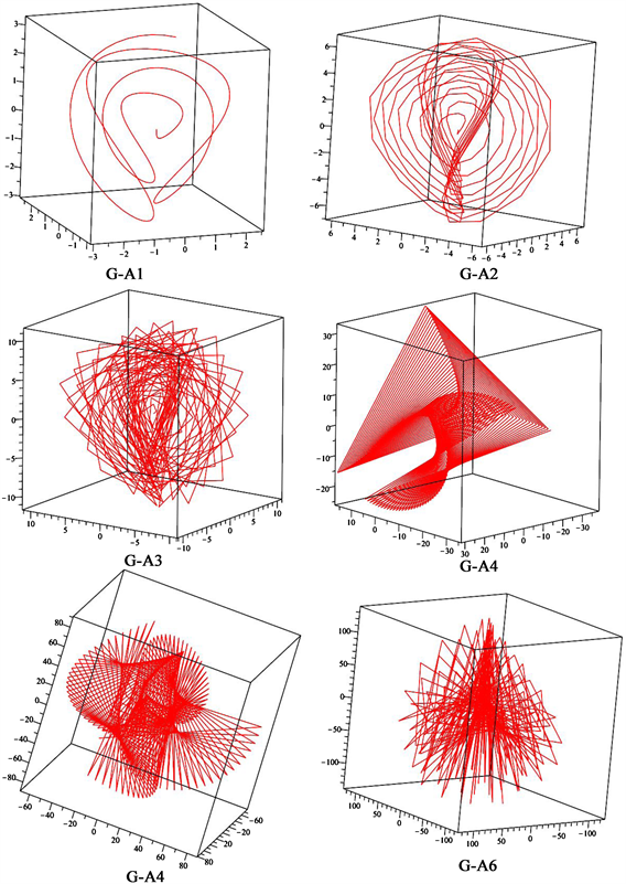
The parameter values and the range of the variable are shown below, for each of the above auto-parallel curves:

G-A1 $a^1=-1$ , $a^2=1$ , $a^3=2$ , $b^1=1$ , $b^2=0$ , $b^3=1$ , $t\in \left[-\mathrm{10,1}\right]$ .

G-A2 $a^1=-1$ , $a^2=1$ , $a^3=2$ , $b^1=1$ , $b^2=0$ , $b^3=1$ , $t\in \left[-\mathrm{50,1}\right]$ .

G-A3 $a^1=-1$ , $a^2=1$ , $a^3=2$ , $b^1=1$ , $b^2=0$ , $b^3=1$ , $t\in \left[-\mathrm{150,1}\right]$ .

G-A4 $a^1=-1$ , $a^2=1$ , $a^3=2$ , $b^1=1$ , $b^2=0$ , $b^3=1$ , $t\in \left[-\mathrm{1500,1}\right]$ .

G-A5 $a^1=-1$ , $a^2=1$ , $a^3=2$ , $b^1=1$ , $b^2=0$ , $b^3=1$ , $t\in \left[-\mathrm{9000,1}\right]$ .

G-A6 $a^1=-1$ , $a^2=1$ , $a^3=2$ , $b^1=1$ , $b^2=0$ , $b^3=1$ , $t\in \left[-\mathrm{19700,1}\right]$ .

G-A7 $a^1=-1$ , $a^2=1$ , $a^3=2$ , $b^1=1$ , $b^2=0$ , $b^3=1$ , $t\in \left[-\mathrm{19800,1}\right]$ .

G-A8 $a^1=-1$ , $a^2=1$ , $a^3=2$ , $b^1=1$ , $b^2=0$ , $b^3=1$ , $t\in \left[-\mathrm{19900,1}\right]$ .

G-A9 $a^1=-1$ , $a^2=1$ , $a^3=2$ , $b^1=1$ , $b^2=0$ , $b^3=1$ , $t\in \left[-\mathrm{19970,1}\right]$ .

G-A10 $a^1=-1$ , $a^2=1$ , $a^3=2$ , $b^1=1$ , $b^2=0$ , $b^3=1$ , $t\in \left[-\mathrm{19990,1}\right]$ .

G-A11 $a^1=-1$ , $a^2=1$ , $a^3=2$ , $b^1=1$ , $b^2=0$ , $b^3=1$ , $t\in \left[-\mathrm{30000000,1}\right]$ .

G-A12 $a^1=-1$ , $a^2=1$ , $a^3=2$ , $b^1=1$ , $b^2=0$ , $b^3=1$ , $t\in \left[-\mathrm{3000000000,1}\right]$ .

G-A13 $a^1=-1$ , $a^2=1$ , $a^3=2$ , $b^1=1$ , $b^2=0$ , $b^3=1$ , $t\in \left[-\mathrm{30000000000,1}\right]$ .

G-A14 $a^1=-1$ , $a^2=1$ , $a^3=2$ , $b^1=1$ , $b^2=0$ , $b^3=1$ , $t\in \left[-\mathrm{300000000000,1}\right]$ .

G-A15 $a^1=-1$ , $a^2=1$ , $a^3=2$ , $b^1=1$ , $b^2=0$ , $b^3=1$ , $t\in \left[-\mathrm{5000000000,1}\right]$ .

G-A16 $a^1=-1$ , $a^2=1$ , $a^3=2$ , $b^1=1$ , $b^2=0$ , $b^3=1$ , $t\in \left[-\mathrm{123456789,1}\right]$ .

G-A17 $a^1=-1$ , $a^2=1$ , $a^3=2$ , $b^1=1$ , $b^2=0$ , $b^3=1$ , $t\in \left[-\mathrm{666,1}\right]$ .

G-A18 $a^1=-1$ , $a^2=10$ , $a^3=2$ , $b^1=1$ , $b^2=0$ , $b^3=1$ , $t\in \left[-\mathrm{11,1}\right]$ .

G-A19 $a^1=-1$ , $a^2=1$ , $a^3=200000$ , $b^1=1$ , $b^2=0$ , $b^3=1$ , $t\in \left[-\mathrm{11,1}\right]$ .

G-A20 $a^1=-1$ , $a^2=1$ , $a^3=499999999$ , $b^1=1$ , $b^2=0$ , $b^3=1$ , $t\in \left[-\mathrm{11,1}\right]$ .

Appendix B

We include 20 graphs of the auto-parallel curves $\gamma$ of ${\nabla }^{\prime }$ , from Subsection 4.2. The pictures show some “global” (“large scale”) behavior, which must be compared with the “local” one in Figure 5 and Figure 6 and to the similar ones in Appendix A.

The parameters values and the variable interval of G-Bn are the same as for G-An in Appendix A, with $n=\overline{1,20}$ .

Appendix C

The non-null Christoffel’s symbols of the metric $\tilde{g}$ are:

${\tilde{\Gamma }}_{22}^2=\frac{1}{r},{\tilde{\Gamma }}_{11}^7=\frac{3}{q-s^3},{\tilde{\Gamma }}_{12}^7={\tilde{\Gamma }}_{21}^7=-\frac{2}{r},$

${\tilde{\Gamma }}_{17}^7={\tilde{\Gamma }}_{71}^7=-\frac{3}{q-s^3},{\tilde{\Gamma }}_{27}^7={\tilde{\Gamma }}_{72}^7=\frac{2}{r},{\tilde{\Gamma }}_{77}^7=\frac{3}{q-s^3}.$

The parameterization of an arbitrary geodesic of $\tilde{g}$ has the form

$\tilde{\beta }\left(t\right)=\left(a^{1}t+b^1,\sqrt{a^{2}t+b^2},a^{3}t+b^3,\cdots ,a^{6}t+b^6,s^3\left(t\right)\right),$

with arbitrary constants $a^i$ and $b^i$ , $i=\overline{1,6}$ . The seventh component $s^3=s^3\left(t\right)$ is a solution of the second-order ODE

$z^{″}+\frac{3{\left(a^1\right)}^2}{a^{1}t+b^1-z}-\frac{2a^1}{a^{2}t+b^2}-\frac{6a^1}{a^{1}t+b^1-z}{z}^{\prime }+\frac{4}{a^{2}t+b^2}{z}^{\prime }+\frac{3}{a^{1}t+b^1-z}{\left(z^{\prime }\right)}^2=0,$

and depends on two more constants (say $a^7$ and $b^7$ ).

Remark C1. (i) All the geodesics $\tilde{\beta }$ are non-complete.

(ii) The 3D projection $\beta =\beta \left(t\right)$ of $\tilde{\beta }$ onto the “visible” Universe with spherical coordinates is not a geodesic anymore, because $\tilde{g}$ does not project onto a 3D metric. However, it is remarkable that the curves $\beta$ are exactly the auto-parallel curves of the connection $\nabla$ , partially depicted in Figure 3, Figure 4 and Appendix A.

The non-null Christoffel’s symbols of the metric $\bar{g}$ are:

${\bar{\Gamma }}_{11}^1=-{\bar{\Gamma }}_{17}^1=-{\bar{\Gamma }}_{71}^1={\bar{\Gamma }}_{77}^1=-{\bar{\Gamma }}_{11}^7={\bar{\Gamma }}_{17}^7={\bar{\Gamma }}_{71}^7=-{\bar{\Gamma }}_{77}^7=-\frac{3}{2q-2s^3},$

${\bar{\Gamma }}_{12}^1={\bar{\Gamma }}_{21}^1=-{\bar{\Gamma }}_{27}^1=-{\bar{\Gamma }}_{72}^1={\bar{\Gamma }}_{22}^2=-{\bar{\Gamma }}_{12}^7=-{\bar{\Gamma }}_{21}^7={\bar{\Gamma }}_{27}^7={\bar{\Gamma }}_{72}^7=\frac{1}{r}.$

The parameterization of an arbitrary geodesic of $\bar{g}$ has the form

$\bar{\beta }\left(t\right)=\left(q\left(t\right)\mathrm{,}\sqrt{a^{2}t+b^2}\mathrm{,}{a}^{3}t+b^3\mathrm{,}\cdots \mathrm{,}{a}^{6}t+b^6\mathrm{,}{s}^3\left(t\right)\right)\mathrm{,}$

with arbitrary constants $a^i$ and $b^i$ , $i=\overline{2,6}$ . The first component $q=q\left(t\right)$ and the seventh component $s^3=s^3\left(t\right)$ are solutions of complicated second-order ODEs, which we could not solve; they depend on four more constants (say $a^1$ , $b^1$ and $a^7$ , $b^7$ ).

Remark C2. (i) All the geodesics $\bar{\beta }$ are non-complete.

(ii) The 3D projection $\epsilon =\epsilon \left(t\right)$ of $\bar{\beta }$ onto the “visible” Universe with spherical coordinates is not a geodesic anymore, because $\bar{g}$ does not project onto a 3D metric. However, it is remarkable that the curves $\epsilon$ are exactly the auto-parallel curves of the connection $\nabla$ , partially depicted in Figure 3, Figure 4 and Appendix A.

Remark C3. The Christoffel’s symbols of $\hat{g}$ are too complicated to be reproduced here. The respective geodesics have parameterized form

$\hat{\beta }\left(t\right)=\left(q\left(t\right)\mathrm{,}r\left(t\right)\mathrm{,}{a}^{3}t+b^3\mathrm{,}\cdots \mathrm{,}{a}^{6}t+b^6\mathrm{,}{s}^3\left(t\right)\right)\mathrm{,}$

with arbitrary constants $a^i$ and $b^i$ , $i=\overline{3,6}$ . The components $q=q\left(t\right)$ , $r=r\left(t\right)$ and $s^3=s^3\left(t\right)$ are solutions of intractable second-order ODEs; they depend on six more constants (say $a^1$ , $b^1$ , $a^2$ , $b^2$ , $a^7$ , $b^7$ ).

The 3D projection $\mu =\mu \left(t\right)$ of $\hat{\beta }$ onto the “visible” Universe with spherical coordinates is not an auto-parallel curve of the connection $\nabla$ , anymore.

Appendix D. On the Gravitational Constant

The gravitational constant has two distinct classes of measurements: 1) based on planetary motion and Cosmological data [61] ; 2) on laboratory experiments, e.g. Cavendish’s torsion balance experiment [51] . Significant variations were registered, without a definitive explanation [52] [53] [54] .

Moreover, the inconsistencies led to expect new phenomena are responsible [62] , beyond the framework of GR with its celebrated equivalence principle inertial mass is proportional to gravitational mass (as a “charge”), a foundational “axiom” of GR, which implies Newton’s Law of Gravity constant is universal:

$m_F~m_G\leftrightarrow G\mathrm{<mo>\; :\; </mo>}\text{Universal}\text{Constant}\mathrm{.}$

The “mystery” regarding the inability to identify a universal constant [62] is consistent with our conclusion Section 2.3.8, mandated by the origin of gravitational charge, as explained in Section 2.2.

D1. Gravity Charge as a Nuclear Spin Polarization Effect

In our use of SM to derive gravity from the quanrk model, gravitational charge is a result of polarization of nuclear spin in the presence of a gravitational field of EM origin (quark fractional charges), of a larger body.

Hence G plays the role of $\epsilon \mathrm{,}\mu$ from maxwell’s EM, but associated with nucleon’s spin, instead of electron spin:

$\text{Electron}\mathrm{<mo>\; :\; </mo>}\text{EM-permitivity}\mathrm{,}\text{permeability}\mathrm{,}\text{Nucleon}\mathrm{<mo>\; :\; </mo>}\text{G-permitivity}\mathrm{.}$

The difference in strength of coupling constants, between electric and magnetic (quark field origin), is measured by the fine structure constant $\alpha$ , approx. 1/137, explaining the difference in ranges for the variability of these coefficients [63] :

$\epsilon ~\mathrm{1..100,}\mu ~\mathrm{10..1000\; <mo>\; ;\; </mo>}\Delta G/G~\mathrm{0.1\; <mi>\; \%\; </mi>\; .}$

The later is much smaller the former two, conjecturally because “natural conditions” do not include the experiments which induce additional polarization (DNO, rotation, supracoductibility etc.).

D2. On Saturation Effects

We can create much stronger permanent magnets in laboratory conditions, with artificial polarization that extends the range of $\epsilon$ and $\mu$ .

The relative limited variability of G could be due to a saturation effect, which is related to the nucleon structure of nuclei, currently not so well understood.

D3. G and DNO, MNR, MRI

It is clear that a much deeper knowledge of solid state physics is needed to understand these aspects, including the theory of DNO, Magnetic Nuclear Resonance, MRI applications etc.

D4. A Statistics Physics Approach

Our attempt to use a partition function approach Section 2.3.3, Ising model 2.3.4, to estimate G, is just a suggestion for physicists to try finding a correlation, as an explanation of the variability of G.

It is beyond the scope of our article to implement a Modified Coulomb Law, to include spin dependence.

nevertheless the analogy with the gravitational tide Section 2.3.1 is illustrative: it holds with van der Wall forces and electric/magnetic polarization, and in view of the fractional electric charges of quarks, must produce a “Zeeman effect/hyperfine split of energy levels”; the problem is “How much”, and if this accounts entirely for Gravity and G.

D5. Spin-Gravity Coupling: Other Studies

The coupling between spin and gravity, in the context of GR is currently studied [64] , as an analog of Stern-Gerlach experiment, but for nuclear spin.

Experimental tests relating spin and gravity are investigated, and Einstein-Cartan Theory used to model it [65] .

In comparison, our work, starting from the quark model of SM which implies such a connection, aims to provide a simpler model: a Modified Coulomb Law and a G-polarization framework. This seems amenable to a direct evaluation of G (theory), in corroboration with the extensive experimental data and Solid State Physics advancements [66] .

In addition to more formal approaches, there seems to be a general trend of thought that Gravity and nuclear spin are in fact related, e.g. [67] .

Considering the specialized literature in a broader context, will benefit the advancement of the theory of gravity, and Science in general, towards a unification with the other interactions.

Appendix E. On Quantum Cosmology

The evolution of Physics, from Classical to Quantum, can be seen happening in other areas of Sciences, notably for our present subject, in Cosmology.

E1. Hawking Laws of BH

Arguably, Beckenstein (1972) and Hawking (1974) played in Cosmology the role of Planck in Physics, introducing the concept of entropy, as if the BH has discrete quantum states, and the BH Radiation, as if behaving like an excited quantum system capable of emission also, together with the BH Laws. This was the result of a thorough study of QM triggered by proposal of Beckenstein regarding the entropy law of BH [68] [69] .

The relation between information/entropy and area, suggested a “quantization at work”. This direction was developed by many researchers, including [70] [71] .

E2. LIGO and Confirmation of GR Prediction

LIGO recent observations Section E2.2 confirmed the gravitational waves prediction of GR, as a “definitive test for General Relativity” [72] (2009).

Yet no theory is “final”, and Einstein stated this about GR. naturally, it has limitations, i.e. physical effects which cannot be accounted for in GR, which we were able to observe, during a century of developments in Physics and Technology (In the Lab and in Astronomy, alike). Ten years later...

E2.1. On Quantum Black-Hole Models

The models from QM, specifically the Bohr’s model of the atom, was recognised as a better model of BHs [71] (see “benefits” within: removing singularity, development of Einstein’s collaborator, N. Rosen’s Theory based on Schrodinger Equation [70] etc.).

Indeed, a BH is a singularity in GR but exhibits internal structure. It therefore is an irreducible system with structure, inviting, because of the entropy concept, related to information paradox and Shannon entropy, to a discrete quantum treatment.

Most notably, the “pre-quantization of BHs”, as a bound, coherent, quantum system, allows to justify Hawking’s Laws, in a manner reminiscent on how Newton’s Theory demonstrated Kepler’s Laws⁷.

E2.2. Gravitational Waves as Scattering Events Quanta?

Dr. Corda’s theory of Quantum Black Holes, based on an analogy with the Bohr’s model of the atom (bound states are quantized), invites further to claim that the merger of two black holes on Sept. 14, 2015, and of two neutron stars on August 17, 2017, should be treated as a scattering event of the two Cosmic-size coherent quantum systems (BH), resulting in a merger (totally similar with a nuclear fusion), and emission of a massive flux of neutrinos (we know not enough to tell if they can escape BHs, being the gauge bosons Spin 1, though, of Gravity as a correction of EM aspect of baryon fields; again, it is a complicated topic, and change of nuclear structure, which involves change in the symmetry group, like in beta decay, may be associated with the Gravitational Waves).

As expected, new advances lead to new ideas and questions: from entropy, treating the irreducible BH system as an “atom” (Ancient Greek and modern meaning), capable of adsorption and radiation in quanta, to a full “scattering theory” picture.

E3. Quantum Gravity from the Standard Model

Our theory emerged from considering the new knowledge about electric charges of electron and proton, revieled by the quark structure: the resolution of the positive charge electric field into a 3-directional, non-isotropic, of mixed signature (neutrons have two negative and one positive), mandates a refinement of Maxwell’s EM, based on pointwise, isotropic and symmetric sources ( $Q\left(e^{-}\right)=-Q\left(p^{+}\right)$ ).

After developing the theory of Gravity of quantum origin (from the quark model of the SM), the first author found the work of Alzofon, confirming experimentally the prediction of the (qualitative) theory etc.

E4. ... and Conversely: From Cosmology to Quantum Physics

The “import” of knowledge and models between Q-Physics in Cosmology, works both ways: the idea/model of Einstein-Rosen wormhole from Cosmology was used in modeling entanglement of in Quantum Physics, and tested on a quantum computer [73] , which can implement teleportation of states via entanglement!

hence, if a BH which appears singular in GR, is a quantum object modeled as an atom, and as a source of Gravity (QBH as “gravitational atom” [71] ), why not compare this framework with the quark model of a Hydrogen atom, as an actual source of gravitational interaction. One would realize that the electric field cannot be isotropic, because of the fractional electric charges of quarks, of opposite signature!

E5. ... and a Question!

It would be interesting to investigate if the GR framework of a Quantized BH, using a metric/differential geometry formalism, is able to reveal additional insight on what the fine structure constant is, which appears from the start in Bohr’s model of the atom [74] [75] .

Appendix F. Inertial Mass vs. Gravitational Mass

The gravitational constant reflects the proportionality between inertial mass $m_F$ (Newton’s Law) and gravitational mass $m_G$ . The later will be referred to as gravitational charge, also denoted as $g_G$ .

F1. Electric Charge with Spin in a Magnetic Field

It is known that in EM the inertial mass to charge ratio $m_F/Q$ determines the dynamics of a particle in an EM field expressed by the Lorentz force, as a first approximation. The spin introduces a torsion to the trajectory, as demonstrated by Stern-Gerlach experiment, with a sign corresponding to the sign of the spin: up or down, relative to the magnetic field. The spin and its own magnetic moment are related as $S=eB$ , hence this effect can be interpreted as a electronic spin-spin interaction, between the sources of the N-S magnet and electron as a mini-magnet.

F2. Gravitational Charge with Spin in a Gravitational Field

It is also speculated, and models built, that mass is of EM origin (a more classical approach), on one hand, or gluon interaction dependent (QCD). Yet quark fields, with gluons as gauge bosons, are SU(2)-gauge Theory fields of EM origin, represented by vector potentials $A_R\mathrm{,}{A}_G\mathrm{,}{A}_B$ as in the spinorial model of the electron (QED).

Hence, it is expected that neutral bodies, with a non-trivial fractional electric structure, as the hydrogen atom, and nuclear spin (neutron, proton) may exhibit a similar behaviour: the ratio $m_F/g_G$ will determine the dynamics in a G-field and a torsion may be present.

F3. Stern-Gerlach Experiment: EM vs. G

If gravity is a side-effect of the internal electric structure and anisotropy of the field of a nucleon⁸, a parallel maybe investigated, as in [64] .

NOTES

¹Considerations based on an extensive research in Mathamtics, Physics and Computer Science [1] .

²... and we owe it to Einstein...

³The same mathematician that developed the theory of differential forms etc.

⁴A String Gauge Theory approach will be developed elsewhere.

⁵In EM: from Faraday to Maxwell-Einstein, back to Coulomb to include spin, then Cartan-Einstein...

⁶Unifications “never worked”: two theories that are too restrictive, cannot be unified, while keeping their foundations unchanged... Maxwell’s Theory is in fact a new framework for field theory, and perhaps a notable exception!

⁷Together with the experimental work of Ticho Brahe, this “trio'' is a very good example of the Scientific Method.

⁸It is usually separated into EM and Strong interaction; but because of our present stage of understanding.

Conflicts of Interest

The authors declare no conflicts of interest regarding the publication of this paper.

References

[1]	Ionescu, L.M. https://about.illinoisstate.edu/lmiones/research/; https://arxiv.org/find/all/1/au:+ionescu_lucian/0/1/0/all/0/1; https://vixra.org/author/lucian_m_ionescu
[2]	Franklin Potter. http://www.sciencegems.com/Icosahedron.html
[3]	Ionescu, L.M. (2019) The Qubit Model: A Platonic and Exceptional Quantum Theory. https://vixra.org/abs/1912.0547
[4]	Ionescu, L.M. (2021) Alzofon-Ionescu Theory of Gravity. https://vixra.org/abs/2106.0056
[5]	Ionescu, L.M. (2022) On Alzofon Experiments of Gravity Control. https://vixra.org/abs/2201.0147
[6]	Ionescu, L.M. (2023) On Antigravity. https://vixra.org/abs/2301.0062
[7]	Hathaway Research International, AGNUE Project. https://www.hathawayresearch.com/portfolios/agnue-anti-gravity-nuclear-entropy/
[8]	Wikipedia, Einstein-Cartan Theory. https://en.wikipedia.org/wiki/Einstein%E2%80%93Cartan_theory
[9]	Ionescu, L.M. (2023) On Emergence of Relativistic Time from Quantum Phase. https://vixra.org/abs/2303.0149
[10]	Ionescu, L.M. (2023) A Quark Fields Emergent Space-Time and Gravity. https://vixra.org/abs/2303.0030
[11]	Merritt, D. (2020) A Philosophical Approach to MOND: Assessing the Milgromian Research Program in Cosmology. Cambridge University Press, Cambridge. https://doi.org/10.1017/9781108610926
[12]	Scholarpedia, “The MOND Paradigm of Modified Dynamics”. http://www.scholarpedia.org/article/The_MOND_paradigm_of_modified_dynamics
[13]	Wikipedia, Scalar-Tensor-Vector Gravity. https://en.wikipedia.org/wiki/Scalar%E2%80%93tensor%E2%80%93vector_gravity
[14]	Falcon Labs. https://www.youtube.com/@FalconSpace
[15]	Ionescu, L.M. (2022) A Note on Dark Matter and Dark Energy. https://vixra.org/abs/2212.0167
[16]	Petrov, A. (2020) Introduction to Modified Gravity. Springer Nature, Cham. https://doi.org/10.1007/978-3-030-52862-1
[17]	Li, B. and Koyama, K. (2020) Modified Gravity. World Scientific Publ., Singapore.
[18]	Koyama, K. (2016) Cosmological Tests on the Modified Gravity. Report of Progress of Physics, 79, Article ID: 046902. https://doi.org/10.1088/0034-4885/79/4/046902
[19]	Ionescu, L.M. (2021) What Gravity Is: Beyond Newton, Einstein, Quantum/Entropy Gravity etc. A VIRequest Project Proposal. https://arxiv.org/pdf/2105.0090v1.pdf
[20]	Schmitt, S. DESY and H1 Spokesperson, and Matthew Wing, University College London and ZEUS Spokesperson. The Most Precise Picture of the Proton. https://cerncourier.com/a/the-most-precise-picture-of-the-proton/
[21]	Riordan, M. (2020, December 23) The Hunting of the Quark. Science. https://orcascurrents.com/the-hunting-of-the-quark/
[22]	Henley, E.M. and Garcia, A. (2007) Subatomic Physics. 3rd Edition, World Scientific, Singapore. http://www.scholarpedia.org/article/Nuclear_Forces https://doi.org/10.1142/6263
[23]	Ionescu, L.M. (2022) Quantum Gravity and Gravity Control. Tesla Extraordinary Conference, Albuquerque, 12 August 2021. https://vixra.org/pdf/2108.0045v1.pdf
[24]	Jehle, H. (1971) Relationship of Flux Quantization to Charge Quantization and the Electromagnetic Coupling Constant. Physical Review D, 3, 306-345. https://doi.org/10.1103/PhysRevD.3.306
[25]	Jehle, H. (1972) Flux Quantization and Particle Physics. Physical Review D, 6, 441-457. https://doi.org/10.1103/PhysRevD.6.441
[26]	Jehle, H. (1975) Flux Quantization and Fractional Charges of Quarks. Physical Review D, 11, 2147-2177. https://doi.org/10.1103/PhysRevD.11.2147
[27]	Jehle, H. (1977) Electron-Muon Puzzle and the Electromagnetic Coupling Constant, Physical Review D, 15, 3727-3759. https://doi.org/10.1103/PhysRevD.15.3727
[28]	Ionescu, L.M. (2022) On Quark Field and Nuclear Physics. https://vixra.org/abs/2212.0217
[29]	Ionescu, L.M. (2023) Why Gravity Cannot Be a Classical Force. https://vixra.org/abs/2301.0096
[30]	Milgrom, M. (2020) MOND vs. Dark Matter in Light of Historical Parallels. Studies in History and Philosophy of Modern Physics, 71, 170-195. https://doi.org/10.1016/j.shpsb.2020.02.004
[31]	Sanders, R.H. (2015) A Historical Perspective on Modified Newtonian Dynamics. Canadian Journal of Physics, 93, 126-138. https://doi.org/10.1139/cjp-2014-0206
[32]	Matt O’Dowd, What If General Relativity Is Wrong? https://www.youtube.com/watch?v=0sTBZ2G4vow
[33]	Ionescu, L.M. (2023) On The Current Physics Crises and the Hierarchy Problem. https://vixra.org/abs/2301.0041m
[34]	Ionescu, L.M. (2022) On the Standard Model, a Note on the Standard Model. https://vixra.org/abs/2212.0195
[35]	Ionescu, L.M. (2023) The Double Slit Experiment. https://vixra.org/abs/2301.0012
[36]	Eckardt, H. (2022) Einstein-Cartan-Evans Unified Field Theory: The Geometrical Basis of Physics, Volume 1: Classical Physics. http://aias.us/documents/uft/TheGeometricalBasisofPhysics.pdf
[37]	Alzofon, F. (2018) Gravity Control with Present Technology (Commentary by David Alzofon).
[38]	Alzofon, F. (1981) Anti-Gravity with Present Technology—Implementation and Theoretical Foundation. AIAA, SAE, and ASME, Joint Propulsion Conference, 17th, Colorado Springs, 27-29 July 1981, 34 p. https://arc.aiaa.org/doi/abs/10.2514/6.1981-1608
[39]	Linder, E.V. (2017) Challenges in Connecting Modified Gravity Theory and Observations. Physical Review D, 95, Article ID: 023518. https://doi.org/10.1103/PhysRevD.95.023518
[40]	Pripoae, G.-T. (2006) Vector Fields Dynamics as Geodesic Motion on Lie Groups. Comptes Rendus de l’Académie des Sciences—Series I, 342, 865-868. https://doi.org/10.1016/j.crma.2006.04.009
[41]	Pripoae, G.-T. and Pripoae, C.-L. (2021) On the Geometrization of Vector Fields (I). Balkan Journal of Geometry and Its Applications, 26, 46-57.
[42]	Tomonaga, S.-I. (1997) The Story of Spin. University of Chicago Press, Chicago.
[43]	Wikipedia, “Electron Magnetic Moment”. https://en.wikipedia.org/wiki/Electron_magnetic_moment
[44]	Vonsovsky, S. (1975) Magnetism of Elementary Particles. Mir Publishers, Moscow.
[45]	Cohen-Tannoudji, C., Diu, B. and Laloe, F. (2020) Quantum Mechanics. 2nd Edition, John Wiley Sons, Hoboken.
[46]	Wikipedia, “Spin”. https://en.wikipedia.org/wiki/Spin_(physics)
[47]	Friedli, S. and Velenik, Y. (2017) Statistical Mechanics of Lattice Systems: A Concrete Mathematical Introduction. Cambridge University Press, Cambridge. https://doi.org/10.1017/9781316882603
[48]	Gao, X., Vaidya, S., Li, K., et al. (2022) Nuclear Spin Polarization and Control in Hexagonal Boron Nitride. Nature Materials, 21, 1024-1028. https://doi.org/10.1038/s41563-022-01329-8
[49]	Hyperphysics, “Nuclear Spin Polarization”. http://hyperphysics.phy-astr.gsu.edu/hbase/Nuclear/spinpol.html
[50]	Dmitriev, A.L. (2008) Measurements of the Influence of Acceleration and Temperature of Bodies on Their Weight. AIP Conference Proceedings, 969, 1163-1169. https://doi.org/10.1063/1.2844956
[51]	Wikipedia, “Gravitational Constant”. https://en.wikipedia.org/wiki/Gravitational_constant
[52]	Anderson, J.D., Schubert, G., Trimble, V. and Feldman, M.R. (2015) Measurements of Newton’s Gravitational Constant and the Length of Day. EPL, 110, 10002. https://doi.org/10.1209/0295-5075/110/10002
[53]	Schlamminger, S., Gundlach, J.H. and Newman, R.D. (2015) Recent Measurements of the Gravitational Constant as a Function of Time. Physical Review D, 91, Article ID: 121101. https://doi.org/10.1103/PhysRevD.91.121101
[54]	Li, Q., et al. (2018) Measurements of the Gravitational Constant Using Two Independent Methods. Nature, 560, 582-588. https://doi.org/10.1038/s41586-018-0431-5
[55]	Perkins, R. (2023) Leonardo da Vinci’s Forgotten Experiments Explored Gravity as a Form of Acceleration. Leonardo, 56, 21-27. https://doi.org/10.1162/leon_a_02322
[56]	Konopinski, E.J. (1978) What the Electromagnetic Potential Describes. American Journal of Physics, 46, 499. https://doi.org/10.1119/1.11298
[57]	Grant, I.S. and Phillips, W.R. (2008) Electromagnetism. 2nd Edition. Manchester Physics. John Wiley & Sons, Hoboken.
[58]	Why Is Nuclear Force Spin Dependent? https://physics.stackexchange.com/questions/288357/why-is-nuclear-force-spin-dependent
[59]	Wang, K.C. and Tsao, H.L. (1945) Relationship between Nuclear Force and Gravitational Force. Nature, 155, 512-513. https://doi.org/10.1038/155512a0
[60]	Xu, J., Li, B.-A., Shen, W.-Q. and Xia, Y. (2015) Dynamical Effects of Spin-Dependent Interactions in Low- and Intermediate-Energy Heavy-Ion Reactions. Frontiers in Physics, 10, Article ID: 102501. https://doi.org/10.1007/s11467-015-0479-8
[61]	Mahto, D., Nadeem, M.S., Prasad, U. and Vineeta, K. (2013) Study of Variation of Gravitational Constant (G) in Very Strong Gravitational Field. International Journal of Astrophysics and Space Science, 1, 56-60. https://article.sciencepublishinggroup.com/pdf/10.11648.j.ijass.20130104.17.pdf https://doi.org/10.11648/j.ijass.20130104.17
[62]	Johnston, H. (2018) Gravitational-Constant Mystery Deepens with New Precision Measurements. Physics World. https://physicsworld.com/a/gravitational-constant-mystery-deepens-with-new-precision-measurements/
[63]	Wikipedia: Relative Permittivity. https://en.wikipedia.org/wiki/Relative_permittivity; https://en.wikipedia.org/wiki/Permeability_(electromagnetism)
[64]	Mashhoon, B. (2021) Gravitomagnetic Stern—Gerlach Force. Entropy, 23, Article No. 445. https://www.mdpi.com/1099-4300/23/4/445
[65]	Kimball, D.F.J. (2023) Testing Gravity’s Effect on Quantum Spins. https://physics.aps.org/articles/v16/80
[66]	Google: “Nuclear Spin Polarization Constants”.
[67]	Edwards, G.T. (2014) Gravitation Maybe Results from Nuclear Magnetic Resonance. https://georgetaitedwards.medium.com/gravitation-maybe-results-from-nuclear-magnetic-resonance-e1c81f342f4
[68]	Beckenstein, J.D. (1998) Quantum Black Holes as Atoms.
[69]	Wikipedia: Black Hole Thermodynamics.
[70]	Rosen, N. (1993) Quantum Mechanics of a Miniuniverse. International Journal of Theoretical Physics, 32, 1435-1440. https://doi.org/10.1007/BF00675204
[71]	Corda, C. and Feleppa, F. (2021) The Quantum Black Hole as a Gravitational Hydrogem Atom. Advances in Theoretical and Mathematical Physics, 1-25. https://arxiv.org/pdf/1912.06478.pdf
[72]	Corda, C. (2009) Interferometric Detection of Gravitational Waves: The Definitive Test for General Relativity. https://arxiv.org/abs/0905.2502
[73]	Walchover, N. (2022) Physicists Create a Holographic Wormhole Using a Quantum Computer. Quanta Magazine. https://arxiv.org/pdf/2302.07897.pdf https://www.quantamagazine.org/physicists-create-a-wormhole-using-a-quantum-computer-20221130/
[74]	Ionescu, L.M. (2023) Our Universe: To Model and to Simulate. https://vixra.org/abs/2305.0162
[75]	Ionescu, L.M. (2023) The Fine Structure Constant Revisited. https://vixra.org/abs/2308.0180