Modeling One Dimensional Two-Cell Model with Tumor Interaction Using Krylov Subspace Methods

Ibtisam Alqahtani^1*, Sharefa Eisa Ali Alhazmi²

¹Umm Al-Qura University Mathematics department, Makkah, Saudi Arabia.
²Department of Mathematics, University College in Qunfudah, Umm Al-Qura University, Makkah, Saudi Arabia.

DOI: 10.4236/am.2023.141002                

Abstract

A brain tumor occurs when abnormal cells grow, sometimes very rapidly, into an abnormal mass of tissue. The tumor can infect normal tissue, so there is an interaction between healthy and infected cell. The aim of this paper is to propose some efficient and accurate numerical methods for the computational solution of one-dimensional continuous basic models for the growth and control of brain tumors. After computing the analytical solution, we construct approximations of the solution to the problem using a standard second order finite difference method for space discretization and the Crank-Nicolson method for time discretization. Then, we investigate the convergence behavior of Conjugate gradient and generalized minimum residual as Krylov subspace methods to solve the tridiagonal toeplitz matrix system derived.

Keywords

PDEs, Krylov Subspace Methods, Finite Difference, Toeplitz Matrix, Two-Cell Model, Tumor Interaction Modeling

1. Introduction

The biological models involving partial differential equations (PDEs) are back to the work of K. Pearson and J. Blakeman in the early 1900s, [1]. In the 1930s others, including R. A. Fisher, applied PDEs to the spatial spread of genes and of diseases, [2] [3]. Population dynamics is a branch of mathematics and ecology that looks at population variations, taking into account the influence of the interactions between populations, [4]. It is necessary that the evolution is continuous in time and Mathematics has a rich history of studying such systems, for example, that is to say governed by differential equations and by the data of an initial state. Mathematical models contain evolutionary partial differential equations (PDEs) arise in diverse domains such as image processing, fluid flow, and computer vision, mechanical systems, relativity, earth sciences, and mathematical finance. The biological invasion is a complicated phenomenon that can be caused by various sources, both natural and unintended, [5]. Like all tumors, the biological and clinical aspects of gliomas are complex and the details of their spatiotemporal growth are still not well understood, [6]. Let $\tilde{u}\left(\tilde{x}\mathrm{,}\tilde{t}\right)$ be the number of cells at a position $\tilde{x}$ and time $\tilde{t}$. We take the basic model, in dimensional form, as a conservation equation [7]:

$\frac{\partial \tilde{u}}{\partial t}\left(\tilde{x},\tilde{t}\right)=\nabla \left(d\nabla \tilde{u}\right)+\rho \tilde{u}+T\tilde{u}$ (1)

$\rho$ represents the net rate of growth of cells including proliferation and death (or loss), T is a matrix representing transfer between sub-populations and d is the diffusion coefficient of cells in brain tissue. The theoretical models, referred to above, considered the brain tissue to be homogeneous so the diffusion and growth rates of the tumor cells are taken to be constant throughout the brain. We consider zero flux boundary conditions on the anatomic boundaries of the brain and the ventricles. So, if D is the brain domain on which the Equation (1) is to be solved, the boundary conditions are $n\cdot d\nabla \tilde{u}$ where $n$ is the unit normal to the boundary $\partial D$ of D. With the geometric complexity of an anatomically accurate brain it is clearly a very difficult analytical problem and a nontrivial numerical problem, even in two dimensions. For simplicity, we limit our study in this paper to the one dimensional problem. In [8], the authors present an extension to Swanson’s reaction diffusion model to include the effects of radiation therapy. In our case, we are motivated to study numerical models that can be used to solve all reaction diffusion equation that describe the propagation of tumor. They inherit traits from the parent tumor and are therefore they capable of vascularize and create new metastases. The cancer is then generalized and finished by threatening the functioning of many vital organs of the patient, so there is a big relationship between growth of tumor cells and biological invasion. The question about modeling cancer tumor growth has led many researchers into extensive studies in this area. This problem has not only fascinated medical and biological researcher, but also applied mathematicians. There have been many techniques developed that can be used to study the evolution and treatment response of the tumor. The tumor growth or decay is considered as a function of time. Moreover, the scientists add a spatial variable to the evolution of the tumor, so that the spread of time will be a function that depends not only on time but also a spatial variable. So, we denote by $u\left(x\mathrm{,}t\right)$ the concentration of tumor cells at position x and time t, then the simulations on growth or decay of tumor cells with time can be studied to understand the phenomena. Since, there are many interactions between sub-populations, so one can look to the existence of two clonal sub-populations u and v within a tumor with mutational transfer. In general case, a clone is a group of identical cells that share a common ancestry, meaning they are produced from a single organism, for more details see [9]. This will help scientists to think for examples where cancer treatment whit medicine is used to kill cancer cells. The existence of two sub-populations u and v within a tumor with mutational transfer needs to be rigorously studied with a focus on the dominance of one sub-population over another. Her initial goal was to simulate and produce a qualitative behavior of the unknown function. Numerical simulation and analytic results of this simpler model will be compared. The plan of the manuscript is the following. Section 2, we describe the model problem that will be solved. In section 3, we present a strategy to compute the analytical solution. Section 4, develops a numerical scheme to obtain a numerical solution that can compared to exact solution. Section 5 study the subpopulation dominates the tumor composition. Finally, we conclude.

2. Problem Setting and Definition

Assume there are two clonal sub-populations within a tumor with mutational transfer. We assume one population has a high growth and low diffusion coefficient while the second population has a low growth rate and high diffusion coefficient; there are different other scenarios we could take. In the model here we do not view the second cell population as a mutation but rather a cell line in its own right. In the following, we describe such a model. The sub-populations are not independent but are connected by mutational events transferring cancer between different cells. A fairly general but basic model to account for population polyclonality is presented in the case of two cell populations:

$\frac{\partial \tilde{u}}{\partial \tilde{t}}\left(\tilde{x},\tilde{t}\right)=d_1\frac{{\partial }^2\tilde{u}}{\partial {\tilde{x}}^2}\left(\tilde{x},\tilde{t}\right)+\left({\rho }_1-\omega \right)\tilde{u}\left(\tilde{x},\tilde{t}\right)$

$\frac{\partial \tilde{v}}{\partial \tilde{t}}\left(\tilde{x},\tilde{t}\right)=d_2\frac{{\partial }^2\tilde{v}}{\partial {\tilde{x}}^2}\left(\tilde{x},\tilde{t}\right)+{\rho }_2\tilde{v}\left(\tilde{x},\tilde{t}\right)+\omega \tilde{v}\left(\tilde{x},\tilde{t}\right)$

$\tilde{u}\left(\tilde{x},0\right)=f(\; x\; ˜\; )$

$\tilde{v}\left(\tilde{x},0\right)=g\left(\tilde{x}\right),\tilde{x}\in ℝ$

with $\tilde{u}$ the more grow rapidly population and $\tilde{v}$ the more rapidly diffusing population, $d_2>d_1$ with ${\rho }_1>{\rho }_2$. Moreover, we assume $\tilde{u}$ cells are the only tumor cells initially present, that $f\left(x\right)>0$ and $g\left(x\right)=0$, with some small probability, $\omega \ll {\rho }_1$, u cells mutate to form $\tilde{v}$ cells. Initially, we suppose there is a source of $\tilde{u}$ tumor cells that have mutated from healthy cells and can multiply rapidly then the neighboring normal cells thereby starting to form a tumor. We can consider of $\omega$ as a measure of the probability of $\tilde{u}$ tumor cells mutating to become the rapidly diffusing tumor cell population $\tilde{v}$.

We first non-dimensionalise the spatially heterogeneous model, which as usual, also decreases the number of effective parameters in the system, and get some idea of the relative importance of various terms.

$x=\sqrt{\frac{{\rho }_1}{d_1}}\tilde{x},t={\rho }_1\tilde{t},\beta =\frac{{\rho }_2}{{\rho }_1}\in \left(0,1\right),\alpha =\frac{\omega }{{\rho }_1},\mu =\frac{d_2}{d_1}$

We define the new function

$u\left(x,t\right)=\frac{d_1}{{\rho }_1\bar{u}}\tilde{u}\left(\sqrt{\frac{{\rho }_1}{d_1}}\tilde{x},{\rho }_1\tilde{t}\right)$ (2)

$v\left(x,t\right)=\frac{d_1}{{\rho }_1\bar{u}}\tilde{v}\left(\sqrt{\frac{{\rho }_1}{d_1}}\tilde{x},{\rho }_1\tilde{t}\right)$ (3)

where $\bar{u}$ represents the initial number of tumor cells in the brain at model time $\tilde{t}=0$.

Let us take the initial source of u tumor cells to be $u\left(x,0\right)=\delta \left(x\right)$ and $v\left(x,0\right)=0$. Where $\delta \left(x\right)$ is the delta function is referred to the Dirac delta function [10].

Therefore, we solve the following problem

$\frac{\partial u}{\partial t}\left(x,t\right)=\frac{{\partial }^{2}u}{\partial x^2}\left(x,t\right)+\left(1-\alpha \right)u\left(x,t\right)$ (4)

$\frac{\partial v}{\partial t}\left(x,t\right)=\mu \frac{{\partial }^{2}v}{\partial x^2}\left(x,t\right)+\beta v\left(x,t\right)+\alpha u\left(x,t\right)$

$u\left(x,0\right)=\delta \left(x\right),$

$v\left(x,0\right)=0,x\in ℝ$

The two cell populations, $u\left(x\mathrm{,}t\right)$ and $v\left(x\mathrm{,}t\right)$ were obtained by the numerical integration of the model system. With this model the parameters are the diffusion coefficient, $d_1\mathrm{,}{d}_2$, the two growth rates ${\rho }_1$ and ${\rho }_2$ of the first and second cell populations respectively. The total density of cancerous cells, $c\left(x,t\right)=u\left(x,t\right)+v\left(x,t\right)$ was obtained by the numerical solution.

3. Analytical Solution

Since, we deal with a linear PDEs, defined in an infinite spatial domain. In 1, we give the analytical solution of (4).

Proposition 1. The solution of (4) is given by

$u\left(x,t\right)={\text{e}}^{\frac{\left(-4\alpha +4\right)t^2-x^2}{4t}}\frac{1}{\sqrt{4\pi t}}$

$v\left(x\mathrm{,}t\right)=\frac{\alpha {\text{e}}^{\frac{\mu \left(1-\alpha \right)-\beta }{\mu -1}t}}{4\sqrt{\left(1-\alpha -\beta \right)\left(\mu -1\right)}}\left({\text{e}}^{-\sqrt{\frac{1-\alpha -\beta }{\mu -1}}x}{v}_1\left(x\mathrm{,}t\right)+{\text{e}}^{\sqrt{\frac{1-\alpha -\beta }{\mu -1}}x}{v}_2\left(x\mathrm{,}t\right)\right)$

where

$v_1\left(x\mathrm{,}t\right)=\text{erfc}\left(\frac{2\sqrt{\frac{-\alpha -\beta +1}{\mu -1}}t-x}{\sqrt{4t}}\right)-\text{erfc}\left(\frac{2\sqrt{\frac{-\alpha -\beta +1}{\mu -1}}\mu t-x}{\sqrt{4\mu t}}\right)$ (5)

$v_2\left(x\mathrm{,}t\right)=\text{erfc}\left(\frac{2\sqrt{\frac{-\alpha -\beta +1}{\mu -1}}t+x}{\sqrt{4t}}\right)-\text{erfc}\left(\frac{2\sqrt{\frac{-\alpha -\beta +1}{\mu -1}}\mu t+x}{\sqrt{4\mu t}}\right)$ (6)

with $\mu >1,1-\alpha -\beta >0$ and erfc is the complementary error function.

Proof. The equation

$\frac{\partial }{\partial t}u\left(x,t\right)=\frac{{\partial }^2}{\partial x^2}u\left(x,t\right)+\left(1-\alpha \right)u\left(x,t\right),-\infty <x<\infty$ (7)

is a second order linear partial differential equation that can be solved using the initial data $u\left(x,0\right)=\delta \left(x\right)$. We use a Fourier transform in the spatial variable x to solve this equation.

Starting with Equation (7), we take Fourier transforms (with respect the space variable x) of both sides, we arrive to

$\frac{\partial }{\partial t}\hat{u}\left(k,t\right)=\left(1-\alpha -k^2\right)\hat{u}\left(k,t\right)$ (8)

The initial condition gives $\hat{u}\left(k,0\right)=\widehat{\delta \left(x\right)}=1$.

Thus the solution is

$\hat{u}\left(k,t\right)={\text{e}}^{\left(1-\alpha -k^2\right)t}={\text{e}}^{\left(1-\alpha \right)t}{\text{e}}^{-k^{2}t}$ (9)

Now, to retrieve $u\left(x\mathrm{,}t\right)$, we have to take the inverse Fourier transform of both sides. Using that the inverse Fourier of Gaussian function us given by $g\left(x,t\right)=\sqrt{\frac{\pi }{t}}{\text{e}}^{-\frac{x^2}{4t}}$ this lead to

$u\left(x\mathrm{,}t\right)=\frac{1}{\sqrt{4\pi t}}{\text{e}}^{\left(1-\alpha \right)t-\frac{x^2}{4t}}$

Since, $u\left(x\mathrm{,}t\right)$ is obtained, now we can solve the second partial differential equation to find v. More precisely, we solve

$\frac{\partial }{\partial t}v\left(x\mathrm{,}t\right)=\mu \frac{{\partial }^2}{\partial x^2}v\left(x\mathrm{,}t\right)+\beta v\left(x\mathrm{,}t\right)+\alpha u\left(x\mathrm{,}t\right)$ (10)

$v\left(x\mathrm{,0}\right)=\mathrm{0,}x\in ℝ$

Once, again we use the Fourier transform in the spatial variable x to solve this equation, we have

$\widehat{\frac{\partial }{\partial t}}v\left(x\mathrm{,}t\right)=\widehat{\mu \frac{{\partial }^2}{\partial x^2}v\left(x\mathrm{,}t\right)}+\widehat{\beta v\left(x\mathrm{,}t\right)}+\widehat{\alpha u\left(x\mathrm{,}t\right)}$

This leads to

$\frac{\partial }{\partial t}V\left(w,t\right)=\mu {\left(iw\right)}^{2}V\left(w,t\right)+\beta V\left(w,t\right)+\alpha U\left(w,t\right)$ (11)

$\frac{\partial }{\partial t}V\left(w,t\right)=\left(\beta -\mu w^2\right)V\left(w,t\right)+\alpha U\left(w,t\right)$ (12)

where $V\left(w,t\right)=\widehat{v\left(x,t\right)}$, and $U\left(w,t\right)=\widehat{u\left(x,t\right)}$.

Using that

$U\left(w,t\right)={\text{e}}^{\left(1-\alpha -w^2\right)t}$

then we arrive to

$\frac{\partial }{\partial t}V\left(w,t\right)=\left(\beta -\mu w^2\right)V\left(w,t\right)+\alpha {\text{e}}^{\left(1-\alpha -w^2\right)t}$

Thus, one again we obtain a first order non-homogeneous ODE in t. Since, $v\left(x,0\right)=0$ then $V\left(w,0\right)=0$. Thus, we have a solve

$\frac{\partial }{\partial t}V\left(w\mathrm{,}t\right)=\left(\beta -\mu w^2\right)V\left(w\mathrm{,}t\right)+\alpha {\text{e}}^{\left(1-\alpha -w^2\right)t}$ (13)

$V\left(w,0\right)=0$ (14)

Using integration factor methods, we get

$V\left(w,t\right)=\alpha {\text{e}}^{\left(\beta -\mu w^2\right)t}{\displaystyle {\int }_0^t}{\text{e}}^{-\left(\beta -\mu w^2\right)s}{\text{e}}^{\left(1-\alpha -w^2\right)s}\text{d}s$

Therefore, we arrive to

$\begin{array}{c}V\left(w,t\right)=\alpha \frac{{\text{e}}^{\left(1-\alpha -w^2\right)t}-{\text{e}}^{\left(\beta -\mu w^2\right)t}}{1-\alpha -\beta +w^2\left(\mu -1\right)}\\ =\alpha \left({\text{e}}^{\left(1-\alpha -w^2\right)t}-{\text{e}}^{\left(\beta -\mu w^2\right)t}\right)\frac{1}{1-\alpha -\beta +w^2\left(\mu -1\right)}\end{array}$ (15)

Now, to retrieve $v\left(x\mathrm{,}t\right)$, we have to take the inverse Fourier transform of both sides. Therefore,

$v\left(x,t\right)={\mathcal{F}}^{-1}\left(V\left(w,t\right)\right)$

The right-hand side of Equation (15) becomes a product of Fourier transforms. Using the convolution theorem properties we have:

$v\left(x,t\right)=\alpha {\mathcal{F}}^{-1}\left\{{\text{e}}^{\left(1-\alpha -w^2\right)t}-{\text{e}}^{\left(\beta -\mu w^2\right)t}\right\}\star {\mathcal{F}}^{-1}\left\{\frac{1}{1-\alpha -\beta +w^2\left(\mu -1\right)}\right\}$

$v\left(x,t\right)=\alpha \left({\mathcal{F}}^{-1}\left\{{\text{e}}^{\left(1-\alpha -w^2\right)t}\right\}-{\mathcal{F}}^{-1}\left\{{\text{e}}^{\left(\beta -\mu w^2\right)t}\right\}\right)\star {\mathcal{F}}^{-1}\left\{\frac{1}{1-\alpha -\beta +w^2\left(\mu -1\right)}\right\}$

$v\left(x,t\right)=\alpha \left({\text{e}}^{\left(1-\alpha \right)t}{\mathcal{F}}^{-1}\left\{{\text{e}}^{-w^{2}t}\right\}-{\text{e}}^{\beta t}{\mathcal{F}}^{-1}\left\{{\text{e}}^{-\mu w^{2}t}\right\}\right)\star {\mathcal{F}}^{-1}\left\{\frac{1}{1-\alpha -\beta +w^2\left(\mu -1\right)}\right\}$

$v\left(x,t\right)=\alpha \left({\text{e}}^{\left(1-\alpha \right)t}\frac{1}{\sqrt{4\pi t}}{\text{e}}^{-\frac{x^2}{4t}}-{\text{e}}^{\beta t}\frac{1}{\sqrt{4\pi \mu t}}{\text{e}}^{-\frac{x^2}{4\mu t}}\right)\star {\mathcal{F}}^{-1}\left\{\frac{1}{1-\alpha -\beta +w^2\left(\mu -1\right)}\right\}$

A straightforward calculus gives

${\mathcal{F}}^{-1}\left\{\frac{1}{1-\alpha -\beta +w^2\left(\mu -1\right)}\right\}=\frac{1}{\mu -1}\frac{1}{2\theta }{\text{e}}^{-\theta \left|x\right|}\mathrm{,}{\theta }^2=\frac{1-\alpha -\beta }{\mu -1}$ (16)

So, we arrive to

$v\left(x,t\right)=\alpha {\text{e}}^{\left(1-\alpha \right)t}\frac{1}{\sqrt{4\pi t}}{\text{e}}^{-\frac{x^2}{4t}}\star \frac{1}{\mu -1}\frac{1}{2\theta }{\text{e}}^{-\theta \left|x\right|}-\alpha {\text{e}}^{\beta t}\frac{1}{\sqrt{4\pi \mu t}}{\text{e}}^{-\frac{x^2}{4\mu t}}\star \frac{1}{\mu -1}\frac{1}{2\theta }{\text{e}}^{-\theta \left|x\right|}$

$\begin{array}{c}v\left(x,t\right)=\frac{\alpha }{2\left(\mu -1\right)\theta }\frac{1}{\sqrt{4\pi t}}{\text{e}}^{\left(1-\alpha \right)t}{\displaystyle {\int }_{\infty }^{+\infty }}{\text{e}}^{-\frac{{\left(x-\varsigma \right)}^2}{4t}}{\text{e}}^{-\theta \left|\varsigma \right|}\text{d}\varsigma \\ -\frac{\alpha }{2\left(\mu -1\right)\theta }\frac{1}{\sqrt{4\pi \mu t}}{\text{e}}^{\beta t}{\displaystyle {\int }_{\infty }^{+\infty }}{\text{e}}^{-\frac{{\left(x-\varsigma \right)}^2}{4\mu t}}{\text{e}}^{-\theta \left|\varsigma \right|}\text{d}\varsigma \end{array}$

So, it is enough to compute the integral ${\displaystyle {\int }_{\infty }^{+\infty }}{\text{e}}^{-\frac{{\left(x-\varsigma \right)}^2}{4t}}{\text{e}}^{-\theta \left|\varsigma \right|}\text{d}\varsigma$. A straightforward calculus give

${\displaystyle {\int }_{\infty }^{+\infty }}{\text{e}}^{-\frac{{\left(x-\varsigma \right)}^2}{4t}}{\text{e}}^{-\theta \left|\varsigma \right|}\text{d}\varsigma =\sqrt{\pi t}{\text{e}}^{{\theta }^{2}t}\left({\text{e}}^{\theta x}\text{erfc}\left(\frac{x+2t\theta }{2\sqrt{t}}\right)+{\text{e}}^{-\theta x}\text{erfc}\left(\frac{2t\theta -x}{2\sqrt{t}}\right)\right)$

Thus, substituting t by $\mu t$ we get

${\displaystyle {\int }_{\infty }^{+\infty }}{\text{e}}^{-\frac{{\left(x-\varsigma \right)}^2}{4\mu t}}{\text{e}}^{-\theta \left|\varsigma \right|}\text{d}\varsigma =\sqrt{\pi \mu t}{\text{e}}^{{\theta }^2\mu t}\left({\text{e}}^{\theta x}\text{erfc}\left(\frac{x+2t\mu \theta }{2\sqrt{\mu }t}\right)+{\text{e}}^{-\theta x}\text{erfc}\left(\frac{-x+2t\mu \theta }{2\sqrt{\mu }t}\right)\right)$

Finally, collecting the above pieces we conclude that

$v\left(x\mathrm{,}t\right)=\frac{\alpha {\text{e}}^{\frac{\mu \left(1-\alpha \right)-\beta }{\mu -1}t}}{4\sqrt{\left(1-\alpha -\beta \right)\left(\mu -1\right)}}\left({\text{e}}^{-\sqrt{\frac{1-\alpha -\beta }{\mu -1}}x}{v}_1\left(x\mathrm{,}t\right)+{\text{e}}^{\sqrt{\frac{1-\alpha -\beta }{\mu -1}}x}{v}_2\left(x\mathrm{,}t\right)\right)$ (17)

with

● $v_1\left(x\mathrm{,}t\right)=\text{erfc}\left(\frac{2\theta t-x}{\sqrt{4t}}\right)-\text{erfc}\left(\frac{2\theta \mu t-x}{\sqrt{4\mu t}}\right)$

● $v_2\left(x\mathrm{,}t\right)=\text{erfc}\left(\frac{2\theta t+x}{\sqrt{4t}}\right)-\text{erfc}\left(\frac{2\theta \mu t+x}{\sqrt{4\mu t}}\right)$

Hence, the request result.

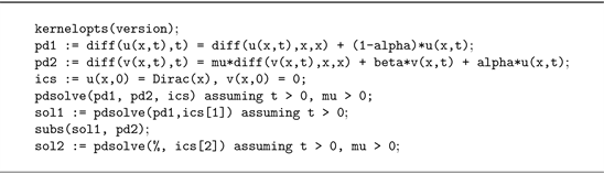
Note that Maple is unable solve the system symbolically. The first PDE has only the unknown u, so we solve it for u, then, we substitute the result in the second PDE, and solve that for v. Using this the following MAPLE lines, once again the analytical solution can be derived.

4. Numerical Simulation

If we hope to solve a PDEs on a computer, we can only do so in an approximate sense, since a computer can only deal with a finite amount of data. The strategy of turning a continuous equation into a finite-dimensional equation suitable for solving on a computer is referred to as discretizing an equation. The most popular being finite differences, finite elements and finite volume discretizations. A common point to these approaches is that at the end, the partial differential equation is converted into a set of linear equations or possible nonlinear equations, that can be solved using different schemes. We will focus in our study on finite difference method.

4.1. Finite Difference Approximations

Since numerical simulation using MATLAB only understands finite domains, we will compute a numerical solution in the one space interval $\left(-a\mathrm{,}a\right)\subset ℝ$ where a is large positive number. Considering the space domain an interval $\left(-a\mathrm{,}a\right)$, $a>0$. The computational domain will be $\left(x\mathrm{,}t\right)\in \left(-a\mathrm{,}a\right)\times \left(\mathrm{0,}T\right)$. The computational domain is discretised into a uniform mesh.

The finite difference grid points (or nodes) are given by

$x_i=-a+i\cdot h,i=0,1,\cdots ,N,h=\frac{2a}{N},$

$t_j=j\cdot \Delta t,j=0,1,\cdots ,N_t,\delta t=\frac{T}{N_t}.$

Let $u_{i\mathrm{,}j}$ (resp $v_{i\mathrm{,}j}$ ) be an approximation to $u\left(x_i\mathrm{,}{y}_j\right)$ (resp. $v\left(x_i\mathrm{,}{y}_j\right)$ ).

The implicit scheme Crank-Nicolson difference equations of our problem are:

$u_j^{n+1}=u_j^n+\frac{\lambda }{2}\left(u_{j+1}^n-2u_j^n+u_{j-1}^n\right)+\frac{\lambda }{2}\left(u_{j+1}^{n+1}-2u_j^{n+1}+u_{j-1}^{n+1}\right)+\delta t\left(1-\alpha \right)u_j^n$

$v_j^{n+1}=v_j^n+\frac{\lambda \mu }{2}\left(v_{j+1}^n-2v_j^n+v_{j-1}^n\right)+\frac{\lambda \mu }{2}\left(v_{j+1}^{n+1}-2v_j^{n+1}+v_{j-1}^{n+1}\right)+\delta t\beta v_j^n+\delta t\alpha u_j^n$

where $\lambda =\frac{\delta t}{h^2}$. In order, to get the solution we add initial conditions: $u_i^0=\delta \left(x_i\right)$ and $v_i^0=0$. The solution vanishes at infinity, so we will use zero boundary conditions at $x=\pm a$. Rearranging the equation, the Crank-Nicolson has the more convenient and condensed symbolic representation (matrix form):

$\left(2I-\lambda \mathcal{A}\right)U^{n+1}=\left(\left(2+2\delta t\left(1-\alpha \right)\right)I+\lambda \mathcal{A}\right)U^n+F^{n+1},n=0,\cdots ,N_t-1.$ (18)

where

$F^{n+1}=\lambda {\left[\begin{array}{c}{u}_0^{n+1}+u_0^n,0,\cdots ,0,u_N^{n+1}+u_N^n\end{array}\right]}^{\text{T}}\in {ℝ}^{N-1}$

$U^{n+1}={\left[u_1^{n+1},u_2^{n+1},\cdots ,u_{N-1}^{n+1}\right]}^{\text{T}}\in {ℝ}^{N-1}.$

and $\mathcal{A}$ is the one-dimensional Laplacian discretization. It is assumed that the boundary values and initial condition are known.

Similarly, we have for $n=0,\cdots ,N_t-1$ :

$\left(2I-\lambda \mu \mathcal{A}\right)V^{n+1}=\left(\left(2+2\delta t\beta \right)I+\lambda \mu A\right)V^n+2\delta t\alpha U^n+G^{n+1}$ (19)

where

$G^{n+1}=\lambda \mu {\left[\begin{array}{c}{v}_0^{n+1}+v_0^n,0,\cdots ,0,v_N^{n+1}+v_N^n\end{array}\right]}^{\text{T}}\in {ℝ}^{N-1}$

$V^{n+1}={\left[v_1^{n+1},v_2^{n+1},\cdots ,v_{N-1}^{n+1}\right]}^{\text{T}}\in {ℝ}^{N-1}.$

For $n=0,\cdots ,N_t-1$, we have

$U^{n+1}={\left(2I-\lambda \mathcal{A}\right)}^{-1}\left\{\left(\left(2+2\delta t\left(1-\alpha \right)\right)I+\lambda \mathcal{A}\right)U^n+F^{n+1}\right\},$ (20)

$V^{n+1}={\left(2I-\lambda \mu \mathcal{A}\right)}^{-1}\left\{\left(\left(2+2\delta t\beta \right)I+\lambda \mu A\right)V^n+2\delta t\alpha U^n+G^{n+1}\right\}.$

So, once the initial condition and boundary conditions are known we can compute using Equation (20) all values at any future time. Moreover, the matrices $2I-\lambda \mathcal{A}$, and $2I-\mu \lambda \mathcal{A}$ are tridiagonal and diagonally dominant, so invertible.

4.2. Krylov Subspace Iteration

We present iterative methods for solving linear algebraic equation based on Krylov subspaces. We use conjugate gradient (CG) method developed by Hestenes and Stiefel in 1950s for symmetric and positive definite matrix and the GMRES method for general non symmetric matrix systems [11]. We fixed the parameter $\alpha =0.5,\beta =0.1$ and $\mu =10$, for a first step, we use Gauss Elimination or LU decomposition to solve the system of algebraic equation, the behavior of $\frac{u}{u+v}$ and $\frac{v}{u+v}$ and $u+v$ is depicted in Figure 1. The Conjugate Gradient method, the Generalized Minimal Residual method are widely used to solve a linear system. The choice of a method depends on $2I-\lambda \mathcal{A}$ symmetry property and or definiteness. Using Conjugate gradient method the solution is obtained and it has the similar behavior as GMRES, see Figure 2. CG is preferable choice in many cases of symmetric-positive-definite matrix because it requires less storage and theoretical bound on convergence rate for CG is double of that GMRES, Figure 3. Moreover, 3 shows the transition of dominance from the rapidly growing u population to the rapidly diffusing v population. The initial tumor consisted of only u cells, for large time the v subpopulation can dominate depending on the value of the mutation probability parameter α. Once again, we observe that the diffusion is more important to glioma growth and invasion then proliferation. The transition of dominance can be interpreted as follows: the total tumor cell population volume is dominated at later times by the second, more aggressive, tumor subpopulation v or v dominates at a single point or neighborhood of points, say, near the center of the tumor, but does not necessarily fill the volume. Figure 4, shows the three dimensional behavior of $\frac{u}{u+v}$ and $\frac{v}{u+v}$. In the simulations, the tumor area increases up to the beginning of the first chemotherapy. As expected, the decrease in the tumor area is larger for a higher value of the effect of the first chemotherapy. The value of the parameters, as well as the initial data of the tumor, are thus critical for determining the spatia-temporal variation of the tumor. There is clearly a maximum value for the tumor area,

(a) (b) (c) (d)

Figure 1. Parameters: $\alpha =0.5,\mu =10$, and $\beta =0.1$, solution behavior $\frac{u}{u+v}$ and $\frac{v}{u+v}$ at different times. (a) Transition of dominance from u to v at t = 50 (s); (b) Transition of dominance from u to v at t = 5 (s); (c) Transition of dominance from u to v at t = 1 (s); (d) Transition of dominance from u to v at t = 0.2 (s).

which is the brain area without the ventricles. An important implication of this solution is that for certain values of α, we see that the initially nonexistent subpopulation v can eventually dominate the growth of the tumor. In our simulation, the different values are fixed so that there is an interaction between two cells, the most significant conditions will be fixed later.

5. Invasion of Tumor Propagation

5.1. Transition of Dominance at a Fixed Location

To see if the subpopulation v dominates the tumor composition at a given location,

(a) (b) (c) (d)

Figure 2. Transition of dominance from u to v at different times with $\alpha =0.5,\mu =10$, and $\beta =0.1$. (a) Transition of dominance from u to v at t = 0.2 (s); (b) Transition of dominance from u to v at t = 1 (s); (c) Transition of dominance from u to v at t = 5 (s); (d) Transition of dominance from u to v at t = 50 (s).

Figure 3. Log₁₀ of absolute error versus time using GMRES and CG schemes.

(a)(b)

Figure 4. Three dimensional behavior of $\frac{u}{u+v}$ and of $\frac{v}{u+v}$. (a) Matlab surf of $\frac{u}{u+v}$ ; (b) Matlab surf of $\frac{v}{u+v}$.

for example at the center of the tumor $x=0$, one can consider the ratio of the two sub-populations $\frac{v\left(x,t\right)}{u\left(x,t\right)}$. Two different periods can be viewed. The first, for small t, the ratio $\frac{v\left(x,t\right)}{u\left(x,t\right)}<1$ since u is initially the only population present. Whereas, for large t, using MAPLE expansion series ( $\frac{v\left(x,t\right)}{u\left(x,t\right)}$, t= infinity, 2) to compute the asymptotic expansion of $\frac{v\left(x,t\right)}{u\left(x,t\right)}$ with respect to the variable t (as t approaches infinity), we get

$\frac{v\left(x,t\right)}{u\left(x,t\right)}=\frac{\alpha }{1-\alpha -\beta }+\frac{1}{2}\frac{\alpha \left(1-\mu \right)}{{\left(1-\alpha -\beta \right)}^2}\frac{1}{t}+O\left(\frac{1}{t^2}\right)$

Thus, we deduce that for large time $\frac{v\left(x,t\right)}{u\left(x,t\right)}\simeq \frac{\alpha }{1-\alpha -\beta }$, therefore the condition for the diffuse population v dominance is $\beta >1-2\alpha$. To estimate the time at which the transition of dominance occurs we solve for t the equation $u/v=1$ we obtain $t^{*}=\frac{1}{2}\frac{\alpha \left(1-\mu \right)}{\left(1-\alpha -\beta \right)\left(1-2\alpha -\beta \right)}$. The time of transition of dominance $t^{\mathrm{<mo>\; *\; </mo>}}$ does depend on $\mu$ and is positive if the condition of dominance is established. If $\mu$ lager than one, the diffusion v cells is important than the u cells and the time dominance is large. Anyway, if the parameters $\alpha$ and $\beta$ satisfy the dominance condition, the time to this transition is short if the diffusion coefficients are nearly equivalent, that is $\mu ~1$.

5.2. Transition of Dominance in Volume

We consider the case in which we can determine the entire tumor and find the proportion of the tumor volume occupied by u and v cells individually. In the present case, transition of dominance arises if the volume occupied by v cells surpass that occupied by u cells. Integrating the solution u and v over $ℝ$, we can find the temporal behavior of the tumor cell subpopulation volumes. Considering $U\left(t\right)$ (resp. $V\left(t\right)$ ) to be the volume of the tumor occupied by u (resp. v) cells, i.e. $U\left(t\right)={\displaystyle {\int }_{ℝ}}u\left(x\mathrm{,}t\right)\text{d}x\mathrm{,}V\left(t\right)={\displaystyle {\int }_{ℝ}}v\left(x\mathrm{,}t\right)\text{d}x$. Using the system of PDEs verified by u and v, we obtain

${\left(\begin{array}{l}U\left(t\right)\hfill \\ V\left(t\right)\hfill \end{array}\right)}^{\prime }=\left(\begin{array}{cc}1-\alpha & 0\\ \beta & \alpha \end{array}\right)\left(\begin{array}{l}U\left(t\right)\hfill \\ V(\; t\; )\hfill \end{array}\right)$

$\left(\begin{array}{l}U\left(0\right)\hfill \\ V\left(0\right)\hfill \end{array}\right)=(\; 1\; 0\; )$

Solving the system we obtain $U\left(t\right)={\text{e}}^{\left(1-\alpha \right)t},V\left(t\right)=\alpha \frac{{\text{e}}^{\left(1-\alpha \right)t}-{\text{e}}^{\beta t}}{1-\alpha -\beta }$. Now, we can deduce the transition of dominance in the volume occurs if the ratio $V/U=1$, this leads to

$t^{\star }=\frac{1}{1-\alpha -\beta }\ln \left(\frac{\alpha }{2\alpha +\beta -1}\right)$

where $1-2\alpha <\beta <1-\alpha$. Certainly, it’s obvious that there are values of $\alpha$ and $\beta$ for which transition of dominance at a point happen and that of volume does not. This can be interpreted as a failure for accurate tumor biopsies. This, let us to conclude that studying a small portion of tissue extracted from the center of a tumor will not necessarily prove the actual total tumor composition.

6. Conclusion

The analytical solution of a coupled system of PDEs is determined using Fourier transform and convolution product. Finite difference method is applied to transform the continuous problem to a system of algebraic equations. An implicit scheme is proposed, more precisely Crank-Nicolson method leads to a special structure system that solved using Krylov subspace. The numerical solution is compared to the analytical solution. Numerical iterative Krylov subspace methods; GMRES and CG are used to solve the implicit linear system. The behavior of tumor propagation over time is studied using different parameters. Finally, a set of numerical experiments confirms the theoretical findings. The transmission of tumor and dominance is developed, and under some condition, the transition of dominance at a point happen and that of volume does not. Considering the results obtained in this paper, we plan in the future to tackle the multi-cell model with tumor Polyclonality in two-dimensional space domain.

Conflicts of Interest

The authors declare no conflicts of interest regarding the publication of this paper.

References

[1]	Clairambault, J. (2013) Partial Differential Equation (PDE), Models. In: Dubitzky, W., Wolkenhauer, O., Cho, K.H. and Yokota, H., Eds, Encyclopedia of Systems Biology, Springer, New York. https://doi.org/10.1007/978-1-4419-9863-7_694
[2]	Fisher, R.A. (1937) The Wave of Advance of Advantageous Genes. Annals of Eugenics (London), 7, 355-369. https://doi.org/10.1111/j.1469-1809.1937.tb02153.x
[3]	Tang, S. and Weber, R.O. (1991) Numerical Study of Fisher’s Equation by a Petrov-Galerkin Finite Element Method. Journal of the Australian Mathematical Society, 33, 27-38. https://doi.org/10.1017/S0334270000008602
[4]	Gurtin, M.E. and MacCamy, R.C. (1977) On the Diffusion of Biological Populations. Mathematical Biosciences, 33, 35-49. https://doi.org/10.1016/0025-5564(77)90062-1
[5]	Lowry, E., Rollinson, E.J., et al. (2012) Biological Invasions: A Field Synopsis, Systematic Review, and Database of the Literature. Ecology and Evolution, 3, 182-196. https://doi.org/10.1016/0025-5564(77)90062-1
[6]	Watkins, S. and Sontheimer, H. (2012) Unique Biology of Gliomas: Challenges and Opportunities. Trends in Neurosciences, 35, 546-556. https://doi.org/10.1016/j.tins.2012.05.001
[7]	Murray, J.D. (1970) On the Gunn Effect and Other Physical Examples of Perturbed Conservation Equations. Journal of Fluid Mechanics, 44, 315-346. https://doi.org/10.1017/S0022112070001854
[8]	Rockne, R., Alvord, E.C., Rockhill Jr, J.K. and Swanson, K.R. (2009) A Mathematical Model for Brain Tumor Response to Radiation Therapy. Journal of Mathematical Biology, 58, 561-578. https://doi.org/10.1007/s00285-008-0219-6
[9]	Cook, R.E. (1983) Clonal Plant Populations. American Scientist, 71, 244-253.
[10]	Buttkus, B. (2000) The Dirac Delta Function and Its Fourier Transform. Spectral Analysis and Filter Theory in Applied Geophysics, Springer, Berlin, Heidelberg. https://doi.org/10.1007/978-3-642-57016-2
[11]	Saad, Y. (2003) Iterative Methods for Sparse Linear Systems. https://www-users.cse.umn.edu/~saad/IterMethBook_2ndEd.pdf