Using the Power Series Method to Evaluate Non-Linear Contingent Claim Partial Differential Equations

Gerald W. Buetow Jr.¹, James Sochacki², Bernd Hanke³

¹BFRC Services, LLC, Irmo, SC, USA.
²James Madison University, Harrisonburg, VA, USA.
³BFRC Services, LLC, Monaco.

DOI: 10.4236/jmf.2022.124039                

Abstract

We use the Power Series Method (PSM) numerical framework for estimating nonlinear variations of the Black-Scholes partial differential equations (PDE). The PSM offers an alternative to using traditional finite difference methods. Traditional approaches often require complicated mathematical manipulations of the nonlinear PDE before they can be deployed; or non-linear relationships are approximated linearly usually involving an iterative solver. The PSM does not have these requirements to be implemented and avoids needing an iterative solver. The PSM allows both symbolic and numerical analysis with full choice of the order of the solver in time. This paper illustrates how the PSM offers an alternative and superior, framework to evaluate nonlinear PDE’s. Several extensions for future research are also offered.

Keywords

Power Series Method, Contingent Claim Valuation, Non-Linear Contingent Claim Partial Differential Equation, Contingent Claim Partial Differential Equation, Symbolic Analysis, Finite Differences, Options Pricing

1. Introduction

Buetow and Sochacki [1] use the PSM approach to evaluate linear PDE generated within the contingent claim valuation framework. Here, we extend their approach to nonlinear PDE (NLPDE). NLPDE occur in contingent claim valuation schemes under various settings. Leland [2] introduced transactional inefficiencies to the original Merton [3] and Black and Scholes [4] frameworks which resulted in a NLPDE. Several variations followed as did approaches to try and solve them. Traditional numerical schemes that solve contingent claim partial differential equations (PDEs) abound in the literature. Our focus here is to extend Buetow and Sochacki [1] into the NLPDE framework; their paper is the first to introduce the Parker and Sochacki [5] [6] Power Series Method (PSM) method within the contingent claim literature.

A contingent claim is a financial asset that has a future payoff contingent on an underlying asset meeting certain criterion. In this paper, we focus on options that have a payoff contingent on the position of the underlying asset relative to a strike price. Traditional valuation frameworks assume that the underlying asset is infinitely liquid; that is, it can be traded with no transaction costs, in infinitesimally small increments, and on a continuum. This assumption is clearly not realistic. Removing it from the valuation process results in altering the valuation framework from a linear PDE to a NLPDE. We will focus on the impact of the liquidity parameter on the valuation estimates to highlight the benefits of using PSM over alternative numerical approaches.

Buetow and Sochacki [1] presented the advantages of the PSM within the contingent claim valuation framework by approximating the plain vanilla PDEs. They illustrate that the PSM approach is inherently more stable than traditional finite difference approaches and so more computationally efficient. PSM is also as accurate as hybrid finite difference approaches like Crank Nicolson and computes a numerical solution more quickly. PSM also is more accurate over a far wider spectrum of time steps than alternative numerical approximation frameworks. Additionally, PSM can be expressed analytically thus enabling the computation of comparative statics (i.e., Greeks) within a far more stable and more accurate environment. Here, we extend their analysis to NLPDEs.

Examples of NLPDE’s in the literature include Amster and Mogni [7], Amster, Averbuj, Mariani, and Rial [8], Bakstein, Howison [9], Barles and Soner [10], Boyle and Vorst [11], Ehrhardt [12], Frey [13], Frey and Patie [14], Frey and Stremme [15], Wilmott [16], and Hoggard, Whaley, and Wilmott [17]. While this is not an exhaustive list, it certainly represents a wide spectrum of frameworks within which a NLPDE results to evaluate contingent claims under various environments where the assumptions of the original Black and Scholes and Merton are relaxed. For our development here we will focus on the NLPDE resulting from transactional inefficiencies as developed by Schonbucher and Wilmott [18], Frey [19], and Liu and Yong [20]. Transactional inefficiencies like illiquidity and trading costs are certainly the most practical. All market participants, both large and small, face these realities when trading, hedging, or replicating contingent claims. Hence, our focus is on this NLPDE.

The aforementioned references focused on developing the necessary mathematics ensuring that the framework met the necessary principles for a solution. Many of these require numerical approaches to enable a solution to be quantified. Other numerical and analytic solutions can be found in Abe and Ishimura [21], Ankudinova and Ehrhardt [22], Anwar and Andallah [23], Arenas, Gonzalez-Parra, and Caraballo [24], Cen and Le [25], Company, Jodar, and Pintos [26], Cont and Voltchkova [27], Duffie [28], Forsyth and Labahn [29], Giles and Carter [30], Gonzalez-Parra, Arenas, and Chen-Charpentier [31], Jandacka and Sevcovic [32], Koleva and Vulkov [33], Kutik and Mikula [34], Lesmana and Wang [20] [35], Sevcovic [36], Sevcovic, Stehlıkova, and Mikula [37], Sevcovic and Zitnanska [38], Wang and Forsyth [39], Zhou, Han, Li, Zhang, and Han [40], Zhou, Li, Wei, and Wen [41], Brennan and Schwartz [42], and Buetow and Sochacki [43] [44] [45]. A good analysis of the Frey model can be found in [19] and Polte [46]. The methodologies and analysis in the above studies often require various transformations into linear approximations of the original NLPDE to be implemented. Our approach here offers what we believe to be a more robust framework for evaluating the NLPDE in the transactional inefficiency environment.

2. Model

Buetow and Sochacki [1] demonstrated that PSM can be used to efficiently solve and analyze the forward linear BS options model and is comparable to the explicit finite difference method and the Crank-Nicolson method. Matić, Radoičić and Stefanica [47] show that PSM can be used to efficiently solve the inverse problem for determining the implied volatility in the linear BS options model. In this paper, we will present how to use PSM to solve and analyze the forward nonlinear BS options model. To be specific, we choose Frey’s model. However, the method presented can easily be extended to other nonlinear BS models.

As in [47], we use auxiliary variables and power series to solve this nonlinear BS options model. In the appendix, we give the symbolic solution for this model similarly to how it was done in [1]. As in [1] and Glover, Duck, Newton [48], we approximate the pay off with a smooth function. We do it to generate a symbolic solution that can be analyzed using calculus including for the “Greeks”. However, since we can also generate polynomials that approximate the solution, one can also use these polynomials to do the same analysis. The symbolic polynomials presented in the appendix were done in the software package Maple.

In [1], we derived methods to approximate the solution to the linear BSOPM using finite differences incorporated with the method of lines to develop a system of ODEs. We then used PSM to approximate the solution to this system of ODEs. This is basically an extension of the Lax-Wendroff method for numerically solving PDEs to higher derivatives. With PSM, this is done automatically (and symbolically) through the computer. In that paper, it was also demonstrated that if the payoff function is approximated with a smooth function one can generate a symbolic solution to the linear BSOPM PDE. In this paper, it will be demonstrated that this can be done for the nonlinear BSOPM PDE through the nonlinearity introduced by [19] and others and developed further by Wilmott. It is very useful that one can generate a symbolic solution to this NLPDE for analysis and numerical evaluation. Evidence of this is presented in the appendix using Maple.

3. Mathematical Framework

Relying on the seminal work of Kyle [49] and employing the classic no arbitrage replication framework commonly found within the option pricing literature, the following NLPDE is easily derived:

$\begin{array}{l}\frac{\partial }{\partial t}V\left(S,t\right)+\frac{1}{2}{\sigma }^2{S}^{2}U\left(S,t\right)\frac{{\partial }^2}{\partial S^2}V\left(S,t\right)+\left(r-q\right)S\frac{\partial }{\partial S}V\left(S,t\right)-rV\left(S,t\right)\\ =F\left(V,S,t\right)\end{array}$ (1)

where the diffusion term U implemented in this paper, which represents the transactional inefficiencies will be

$U\left(S,t\right)={\left(1-\lambda \left(S,t\right)\frac{{\partial }^2}{\partial S^2}V\left(S,t\right)\right)}^a.$

This term introduces the nonlinearity. The value of the option is given by $V\left(S,t\right)$ where S is the value of the underlying asset for the option and t is calendar time. We denote our payoff as $Q\left(S\right)=V\left(S,T\right)$ where T is the maturity time of the option.

Equation (1) has appeared extensively in the literature. Most commonly, the exponent, a, in $U\left(S,t\right)$ is set to −2. We will use that quantification in this work. [18] assume that the function $\lambda \left(S,t\right)$ is a dimensionless constant measuring the liquidity of the market. [19] has a similar form for $\lambda \left(S,t\right)$. [20] define $\lambda \left(S,t\right)$ as $\hat{a}\left(1-{\text{e}}^{-\beta \left(T-t\right)}\right)$ where $\hat{a}$ is a coefficient and a constant that measures the price impact, $\tau =T-t$ is time to expiry and $\beta$ is a decay coefficient. We follow [15] [18] and [19] and assume that $\lambda \left(S,t\right)$ is a constant. [48] present Equation (1) with constant $\lambda \left(S,t\right)$ but include additional insights into its various properties. There is wide acceptance of this form with the most practical implications throughout the industry.

In the linear paper ( [1]), the put¹ payoff function $Q_0\left(S\right)=\max \left(K-S,0\right)$ (where Kis the strike price of the option) was approximated by the smooth function $Q_1\left(S\right)=\ln \left(1+\exp \left(S-K\right)\right)-\left(S-K\right)$. In [48], the put payoff is approximated by $Q_2\left(S\right)=\frac{1}{2}\left(\left(K-S\right)+\sqrt{{\left(K-S\right)}^2+{\rho }^2}\right)$. Letting $\rho \to 0^{+}$ gives a better approximation. Unfortunately, this function is not smooth at $\rho =0$. Therefore, we approximate the put payoff here by $Q_3\left(S\right)=-\frac{1}{2}\left(S-K\right)+\frac{1}{\pi }\left(S-K\right)\arctan \rho \left(S-K\right)-\frac{1}{2\pi \rho }\ln \left({\rho }^2{\left(S-K\right)}^2+1\right)$ which leads to a better approximation of the put payoff as $\rho \to \infty$. All the numerical examples presented in this paper were done using $Q_0$ and $Q_3$ with $\rho =2^{24}$ and gave an answer to within 10⁻⁵ of the results presented.

1For a call, $K-S$ is replaced by $S-K$ and $S-K$ is replaced by $K-S$ in each $Q_i$ for $i=0,1,2,3$.

As shown in the linear paper, one can obtain a symbolic answer using a smooth Q. There we showed how Picard iteration on the integral form of the PDE can generate the power series solution in t or $\tau =T-t$ for the option value V. The same can be done for any of the nonlinear forms for the BSOPM. We provide the PSM outline for doing this for the nonlinear problem done in this work in the appendix where a symbolic solution up to degree 2 in $\tau =T-t$ for any smooth Q, including $Q_3$ is provided. One can use this symbolic form of the solution to analyze the “greeks” of the option. We leave this as an exercise for the reader. In this paper, only the discretized PSM presented in the linear paper will be applied to the nonlinear BSOPM. In the appendix, we give a system of PDEs that can be used to obtain a symbolic (or numeric) power series solution to $V\left(S,\tau \right)$ for any smooth Q.

We also point out that since we have a power series in $\tau$, one can replace $\tau$ by $z\left(\tau \right)$ (or $\tau$ by a power series $\tau \left(z\right)$ ) for any function z to get an expansion of V in powers of z. This allows one to get numerical approximations of V in terms of z or symbolic approximations of V in terms of z.

We will do our numerical derivation in $\tau =T-t$ and consider only the following PDE

$\frac{\partial }{\partial \tau }V=\frac{1}{2}{\sigma }^2{S}^{2}U\left(S,\tau \right)\frac{{\partial }^2}{\partial S^2}V+\left(r-q\right)S\frac{\partial }{\partial S}V-rV;V\left(S,0\right)=Q\left(s\right)$ (2)

where $V\left(S,\tau =T-t\right)$ replaces $V\left(S,t\right)$ in Equation (1). We note again that our derivation can be used for more than the $U\left(S,\tau =T-t\right)$ given above.

4. Setting up the DPSM

We now outline how to obtain a Lax-Wendroff approximation to any degree desired in $\tau$ for Equation (2) with the $U\left(S,\tau \right)$ given above. Hoffman and Frankel [50] and Evans, et al. [51] are both good and thorough introductions to Crank-Nicolson, MOL and Lax Wendroff schemes for linear and nonlinear PDEs. Money [52] presents a thorough demonstration of how PSM with MOL gives a generalization of the Lax Wendroff scheme with error estimates and stability analysis.

We will assume $\lambda \left(S,\tau \right)$ is a constant, but the discretized PSM applies for most forms for $\lambda \left(S,\tau \right)$ in the literature and certainly those discussed above. The derivation would be similar as presented below but with different auxiliary variables. A thorough discussion of auxiliary variables is given in Parker and Sochacki [5] [6] and in Sochacki [53].

We first deal with $U\left(S,\tau \right)$. Note that if x is a power series in z and $y=x^a$ then differentiating leads to

$y^{\prime }=a{x}^{a-1}{x}^{\prime }$

and then

$x{y}^{\prime }=a{x}^a{x}^{\prime }=ay{x}^{\prime }.$ (3)

Using this, it is straightforward to develop the power series coefficients for y. In fact, if

$x=\underset{i=0}{\overset{n}{{\displaystyle \sum }}}{x}_i{z}^i,y=\underset{i=0}{\overset{n}{{\displaystyle \sum }}}{y}_i{z}^i$

then

$x^{\prime }=\underset{i=0}{\overset{n-1}{{\displaystyle \sum }}}\left(i+1\right)x_{i+1}{z}^i,y^{\prime }=\underset{i=0}{\overset{n-1}{{\displaystyle \sum }}}\left(i+1\right)y_{i+1}{z}^i$

and substituting these four power series into Equation (3) gives

$x{y}^{\prime }=\underset{i=0}{\overset{n}{{\displaystyle \sum }}}{x}_i{z}^i\underset{i=0}{\overset{n-1}{{\displaystyle \sum }}}\left(i+1\right)y_{i+1}{z}^i=ay{x}^{\prime }=a\underset{i=0}{\overset{n}{{\displaystyle \sum }}}{y}_i{z}^i\underset{i=0}{\overset{n-1}{{\displaystyle \sum }}}\left(i+1\right)x_{i+1}{z}^i.$

Multiplying out the series using Cauchy products as outlined in the linear paper produces

$\underset{i=0}{\overset{n-1}{{\displaystyle \sum }}}\left(\underset{j=0}{\overset{i}{{\displaystyle \sum }}}\left(j+1\right)y_{j+1}{x}_{i-j}\right)z^i=a\underset{i=0}{\overset{n-1}{{\displaystyle \sum }}}\left(\underset{j=0}{\overset{i}{{\displaystyle \sum }}}\left(j+1\right)x_{j+1}{y}_{i-j}\right)z^i.$

Equating the terms multiplied by like powers of z, and solving for the coefficient $y_{i+1}$ in terms of all the lower coefficients of y provides the recurrence relation for each coefficient of the power series for y. Doing this, gives us

$\underset{i=0}{\overset{n-1}{{\displaystyle \sum }}}\left(\underset{j=0}{\overset{i}{{\displaystyle \sum }}}\left(j+1\right)y_{j+1}{x}_{i-j}\right)z^i=\underset{i=0}{\overset{n-1}{{\displaystyle \sum }}}\left(\underset{j=0}{\overset{i}{{\displaystyle \sum }}}a\left(j+1\right)x_{j+1}{y}_{i-j}\right)z^i$

and then

$\underset{j=0}{\overset{i}{{\displaystyle \sum }}}\left(j+1\right)y_{j+1}{x}_{i-j}=\underset{j=0}{\overset{i}{{\displaystyle \sum }}}a\left(j+1\right)x_{j+1}{y}_{i-j}.$

Rewriting slightly gives us

$\left(i+1\right)y_{i+1}{x}_0+\underset{j=0}{\overset{i-1}{{\displaystyle \sum }}}\left(j+1\right)y_{j+1}{x}_{i-j}=a\underset{j=0}{\overset{i}{{\displaystyle \sum }}}\left(j+1\right)x_{j+1}{y}_{i-j}.$

Solving on the left-hand side for $y_{i+1}$ leads to

$y_{i+1}=\frac{1}{\left(i+1\right)x_0}\left(a\underset{j=0}{\overset{i}{{\displaystyle \sum }}}\left(j+1\right)x_{j+1}{y}_{i-j}-\underset{j=0}{\overset{i-1}{{\displaystyle \sum }}}\left(j+1\right)y_{j+1}{x}_{i-j}\right)$

or after re-indexing

$y_{i+1}=\frac{1}{\left(i+1\right)x_0}\left(a\left(i+1\right)x_{i+1}{y}_0-\underset{j=0}{\overset{i-1}{{\displaystyle \sum }}}\left(j\left(a+1\right)+\left(a-i\right)\right)x_{j+1}{y}_{i-j}\right)$ (4)

This recurrence relation gives all the coefficients of the power series for ${\left(x\left(z\right)\right)}^a$. Since

$U\left(S,\tau \right)={\left(1-\lambda \frac{{\partial }^2}{\partial S^2}V\left(S,\tau \right)\right)}^a$

and PSM gives the power series for $1-\lambda \frac{{\partial }^2}{\partial S^2}V\left(S,\tau \right)$ in $\tau$, we can use the above recurrence relation to obtain the power series for U for any a but in our numerical examples we use $a=-2$. We choose $a=-2$ because this is the result that occurs in the derivation using Ito’s lemma as shown by [19] and many others.

If $a=-2$ then

$U\left(S,\tau \right)={\left(1-\lambda \frac{{\partial }^2}{\partial S^2}V\left(S,\tau \right)\right)}^{-2}$.

Since

$y=\frac{1}{1-x}=1+x+x^2+x^3+\cdots$

for $\left|x\right|<1$, one has that

$y^{\prime }=\frac{1}{{\left(1-x\right)}^2}=y^2=1+2x+3x^2+4x^3+\cdots$

for $\left|x\right|<1$. If

$x=\lambda \frac{{\partial }^2}{\partial S^2}V$

is substituted into Equation (2), the PDE in Equation (2) gives rise to

$\begin{array}{c}\frac{\partial }{\partial \tau }V=\frac{1}{2}{\sigma }^2{S}^{2}U\left(S,\tau \right)\frac{{\partial }^2}{\partial S^2}V+\left(r-q\right)S\frac{\partial }{\partial S}V-rV\\ =\frac{1}{2}{\sigma }^2{S}^2\frac{1}{{\left(1-x\right)}^2}\frac{{\partial }^2}{\partial S^2}V+\left(r-q\right)S\frac{\partial }{\partial S}V-rV\\ =\frac{1}{2}{\sigma }^2{S}^2\left(1+2x+3x^2+\cdots \right)\frac{{\partial }^2}{\partial S^2}V+\left(r-q\right)S\frac{\partial }{\partial S}V-rV.\end{array}$

One can rearrange this last PDE to read as

$\frac{\partial }{\partial \tau }V-\frac{1}{2}{\sigma }^2{S}^2\frac{{\partial }^2}{\partial S^2}V-\left(r-q\right)S\frac{\partial }{\partial S}V+rV=\frac{1}{2}{\sigma }^2{S}^2\left(2x+3x^2+\cdots \right)\frac{{\partial }^2}{\partial S^2}V,$

where the nonlinear terms can now be viewed as $F\left(\frac{{\partial }^2}{\partial S^2}V,\lambda ,S,\tau \right)$ as in Equation (1). This equation shows how sensitive the nonlinearity can become as x gets further from 0 (but stays < 1 in magnitude). (If $x=0$, one obtains the linear Black Scholes contingent claim PDE.) This sensitive nature created by the Frey illiquidity has been noted by other researchers (Heider [54]). However, we believe this is the first paper that studies this nonlinearity in a power series expansion as presented in this last equality. Some of the findings are not intuitive and show the complicated convergence (and stability) regions that arise in numerically solving this nonlinear PDE. We emphasize that the method presented works for $\left|x\right|>1$. However, our study shows that the size of $\left|x\right|$ certainly determines the error, convergence, and stability in the numerical approximations. It probably also reaches to the limits of the nonlinearity to model a real economy.

5. The Discretization Scheme Using PSM

We now layout the finite difference grid for $\left(S,\tau \right)$. This is the same grid as given in the linear paper. We present it here for completeness.

We choose an increment value ∆S for the interval $0\le S\le S_M$ and let $S_i=i\Delta S$ for $i=0,1,2,3,\cdots ,I$ so that $S_0=0$ and $S_I=I\Delta S=S_M$. We determine a power series for $V\left(S_i,\tau \right)$ for each i. To do this, we let $v_i\left(\tau \right)$ be our Maclaurin polynomial approximation to $V\left(S_i,\tau \right)$ and let $W_i^n$ be the value $v_i\left(n\Delta \tau \right)$. The discretized version of Equation (2) is

${v^{\prime }}_i\left(\tau \right)=\frac{1}{2}{\sigma }^2{S}_i^2{u}_i\left(\tau \right)D^2{v}_i\left(\tau \right)+\left(r-q\right)S_{i}D{v}_i\left(\tau \right)-r{v}_i\left(\tau \right)$ (5)

with $v_i\left(0\right)=Q\left(S_i\right)$, $u_i\left(\tau \right)=U\left(S_i,\tau \right)$, D a discretized approximation for $\frac{\partial }{\partial S}$ and $D^2$ a discretized approximation for $\frac{{\partial }^2}{\partial S^2}$. For example, if we use the centered difference approximations

$D{v}_i\left(\tau \right)=\frac{v_{i+1}\left(\tau \right)-v_{i-1}\left(\tau \right)}{2\Delta S},D^2{v}_i\left(\tau \right)=\frac{v_{i+1}\left(\tau \right)-2v_i\left(\tau \right)+v_{i-1}\left(\tau \right)}{\Delta S^2}$

then Equation (5) in discretized form becomes the ODE

$\begin{array}{c}{v^{\prime }}_i\left(\tau \right)=\frac{1}{2}{\sigma }^2{S}_i^2{u}_i(\tau )\left(\frac{v_{i+1}\left(\tau \right)-2v_i\left(\tau \right)+v_{i-1}\left(\tau \right)}{\Delta S^2}\right)\\ +\left(r-q\right)S_i\left(\frac{v_{i+1}\left(\tau \right)-v_{i-1}\left(\tau \right)}{2\Delta S}\right)-r{v}_i\left(\tau \right)\end{array}$ (6)

with

$u_i\left(\tau \right)={\left(1-\lambda \left(\frac{v_{i+1}\left(\tau \right)-2v_i\left(\tau \right)+v_{i-1}\left(\tau \right)}{\Delta S^2}\right)\right)}^{-2}$.

Therefore, if $i=1,2,\cdots ,I$ for some counting number I, we have a system of I IV ODEs that we can solve using PSM. That is, we assume

$v_i\left(\tau \right)=\underset{j=0}{\overset{J}{{\displaystyle \sum }}}{v}_{i,j}{\tau }^j$ (7)

for each i and some user chosen J that determines the degree of the Maclaurin polynomial that approximates $V\left(S,\tau \right)$. We determine the polynomial for $u_i\left(\tau \right)$ using the recurrence relation (4) and the fact that we know the polynomials for $v_{i-1}\left(\tau \right),v_i\left(\tau \right),v_{i+1}\left(\tau \right)$. The standard conditions for numerical solutions to Equation (2) (these are the one used in the linear paper) are used to give values to $v_0\left(\tau \right)$ and $v_{I+1}\left(\tau \right)$. Since the PSM polynomial of degree $J=1$ (PSM 1) is equivalent to EFDM, this PSM algorithm can be used to compare EFDM against PSM J for any user chosen J. It is straightforward to combine the right-hand side of Equation (6) into a power series in $\tau$ after using Cauchy product of two power series to multiply out

$u_i\left(\tau \right)\left(\frac{v_{i+1}\left(\tau \right)-2v_i\left(\tau \right)+v_{i-1}\left(\tau \right)}{\Delta S^2}\right)$.

We can compute the $v_i\left(\tau \right)$ numerically or symbolically using a software package. We present symbolic representations using Maple in the Appendix. Maple was able to generate an 8^th degree symbolic polynomial for each $i=1,\cdots ,32$ in less than two minutes. It did this also for $Q_3\left(S\right)$ but the output is too large to present in this paper. In the Appendix the output is shown for the solution to Equation (2) with $Q_3\left(S\right)$ using Picard iteration in Maple. It is also important to point out that one can replace as many as parameters with numerical values as desired in this symbolic polynomial to study the impact of other parameters in the Greeks. We note that coefficient of $\tau$ has the term ${\left(1-\lambda Y_3\right)}^{-2}$ in it and that this term occurs to more negative exponents in the coefficients of ${\tau }^2$ with larger exponents along with terms in $\lambda$. These contribute to the nonlinear feedback in an illiquid market.

Of course, one can use Equation (7) and discrete approximations for S derivatives to get the greeks numerically to order J.

Using $K=1,\Delta S=0.125,r=0.04,q=0,\sigma =0.2$ and $\lambda =1$ the fourth degree (Maclaurin polynomial) approximation to $v_{20}\left(\tau \right)$ ( $S=20\Delta S=2.5$ ) for a call at $\tau =0$ is

$1.375+0.04\tau -0.0008{\tau }^2+0.000001-0.000000011{\tau }^4$.

Again, it is straightforward for Maple or a computing language to generate higher degree polynomial approximations with the same code. The only number the user must change is J.

In our numerical results, we demonstrate that the explicit FDM gives similar results to PSM under convergence regions but that PSM for $J\ge 2$ has larger (stronger) convergence regions. Most of the results shown with PSM are with $J=2$ but we have verified these results with $J=4$. Since PSM can record any (all) of the Greeks, one can measure any of these quantities during the computing of the solution to determine their impact (size) on the value of the option and/or the error, convergence, stability of the numerical approximations.

6. Modeling Results and Comparisons

2Again, one should note that this payoff function is not everywhere differentiable either and so better alternatives exist. We offer such an approach in the appendix. For our purposes here we are focusing our presentation on a numerical approach such that the concerns associated with the payoff functional form are mitigated within the framework.

Figure 1 and Figure 2 clearly show the instability issues using the traditional explicit FDM approaches as also presented by [48]. The magnitude of the pricing impacts is extraordinarily large and oscillatory. The efficacy of the approach is clearly challenged. Figure 1 illustrates pricing impact oscillations an order of magnitude that are 10⁴ the size of the option prices. Figure 2 shows that the estimated pricing impacts from the feedback in Equation (1) are 10² the size of the option value. These are unacceptable results that simply have no realistic interpretation. The nonlinearities of Equation (1) along with the non-continuous characteristics of the payoff function at $S=K$ are introducing instabilities that can’t be handled by traditional FDM approaches. As explained above the traditional payoff function can produce instabilities in valuation estimates as can be seen in Figure 1 and Figure 2. [48] suggest using the payoff function $Q_2\left(S\right)=\frac{1}{2}\left(\left(K-S\right)+\sqrt{{\left(K-S\right)}^2+{\rho }^2}\right)$ for puts (and $S=K$ for call options).²

Figure 1. Impact of liquidity on put option value using finite differences.

Figure 2. Impact of liquidity on call option value using finite differences.

Figure 1 and Figure 2, despite the clear numerical limitations of FDM, still illustrate some interesting findings. The impact of the feedback parameter when $\lambda$ is greater than 1 is intuitive. As the parameter increases the pricing impact generally increases. If we interpret this parameter as a proxy for liquidity, then this result matches what we expect. That is, as illiquidity increases the impact on the options value should be more significant because the ability to create a hedge increases. As the term $\lambda \frac{{\partial }^2}{\partial S^2}$ approaches 1, the impact on pricing becomes more significant as well. The interplay between these two terms may be at the source of some of the numerical properties presented above.

Figure 1 illustrates the instability of the numerical approximation to a put option as a function of the liquidity parameter when using the finite difference approach to the Equation (2).

Figure 2 illustrates the instability of the numerical approximation to a call option as a function of the liquidity parameter when using the finite difference approach to the Equation (2).

7. PSM Results

Figure 3 and Figure 4 present the results using our PSM approach for Equation (1) under varying feedback constants less than 1 for each option type. PSM eliminates the erratic numerical results found using the FDM. This is an extremely important result. PSM is far more stable. While the general impacts increase with illiquidity, that impact is economically more defensible using PSM than FDM. Also, the impacts are smooth functions with peak impact near $S=K$ where we have the maximum impact of the nonlinearities. For $\lambda <1$ we see a monotonic pricing impact of illiquidity. This can be seen in both Figure 3 for the put option as well as Figure 4 for the call option. Note also, that the boundary issues for the put option entirely disappear using PSM.

Figure 3. Impact of liquidity (<1) on put option value using PSM.

Figure 4. Impact of liquidity (<1) on call option value using PSM.

Figure 3 illustrates that numerical approximation to a put option for small liquidity parameters. Using PSM the approximation does not suffer any instabilities and illustrates that the liquidity parameter has the most impact on valuation around the strike price. Moreover, as the parameter gets larger, the impact on value increases.

Figure 4 illustrates that numerical approximation to a call option for small liquidity parameters. Using PSM the approximation does not suffer any instabilities and illustrates that the liquidity parameter has the most impact on valuation around the strike price. Moreover, as the parameter gets larger, the impact on value increases.

Figure 5 represents the results for the put options and Figure 6 for the call option for values of $\lambda >1$. These results are somewhat counter intuitive but consistent with the findings of [54] except there they artificially avoid the counter-intuitive results by imposing arbitrary properties onto the solution. As $\lambda$ increases to very large values we see that the pricing impact changes sign. Note also, that large $\lambda$ also has larger price impact relative to $\lambda <1$. This is intuitive and matches earlier studies. While the impact is positive, the effect of the parameter matches that of above; larger parameters have larger impact. Monotonicity in both areas is maintained, however, suggesting that the result is not a numerical flaw but a property of the pricing dynamic. Analyzing Equation (1), we observed that the product $\lambda \frac{{\partial }^2}{\partial S^2}$ is introducing larger impacts as it gets closer to 1. The feedback parameter and the gamma term ( $\frac{{\partial }^2}{\partial S^2}V\left(S,t\right)$ ) may be interacting to produce results that increase the price impact more than expected. As the gamma gets larger at the money, the need to hedge the risk-free portfolio becomes far more frequent, so that any illiquidity has a larger impact on valuation. Future study might focus on the details of this interaction using the more robust pricing approach introduced here.

Figure 5 illustrates that numerical approximation to a put option for large liquidity parameters. Using PSM the approximation does not suffer any instabilities and illustrates that the liquidity parameter has the most impact on valuation around the strike price. Interestingly, the impact of the liquidity parameter on valuation changes sign as it increases.

Figure 6 illustrates that numerical approximation to a call option for large liquidity parameters. Using PSM the approximation does not suffer any instabilities and illustrates that the liquidity parameter has the most impact on valuation around the strike price. Interestingly, the impact of the liquidity parameter on valuation changes sign as it increases.

3Presenting payoff graphs for $\lambda <1$ is not useful since for each $\lambda <1$, the payoff profiles are indistinguishable from one another.

Figure 7 and Figure 8 present the price impacts for $\lambda >1$ using the payoff profile for each option type.³ These more traditional graphics are consistent with earlier studies.

Figure 5. Impact of liquidity (>1) on put option value using PSM.

Figure 6. Impact of liquidity (>1) on call option value using PSM.

Figure 7. Impact of liquidity (>1) on put option payoff function using PSM.

Figure 8. Impact of liquidity (>1) on call option payoff function using PSM.

Figure 7 illustrates the impact of the liquidity parameter over a wide spectrum of underlying asset prices. It shows that the PSM approach offers a very smooth approximation across the entire spectrum, as well as illustrating the impact of the parameter on the put option value. As the parameter increases so does its impact on value relative to the Black-Scholes solution.

Figure 8 illustrates the impact of the liquidity parameter over a wide spectrum of underlying asset prices. It shows that the PSM approach offers a very smooth approximation across the entire spectrum, as well as illustrating the impact of the parameter on the call option value. As the parameter increases so does its impact on value relative to the Black-Scholes solution.

8. Conclusion

We have introduced the PSM framework as a viable approach to numerically (or symbolically) analyze the NPDE’s frequently found in the contingent claim valuation literature. To illustrate the strengths of PSM we evaluated a commonly found NPDE where a feedback term is introduced to the dynamics of the riskless hedge portfolio. Many of the shortcomings in other numerical and analytic approaches are avoided when using the PSM approach. It more easily deals with the discreteness found around the strike price which frequently causes many other numerical frameworks to become unstable. PSM can produce a symbolic as well as numeric solution each of which can be analyzed in terms of the Greeks and sensitivity to the solution. We illustrated this impact and the corresponding improvements using PSM. For those interested in a more stable and robust numerical scheme, and one that offers a complete set of first and second order solutions across the entire numerical grid, PSM offers a viable and accurate alternative. Future research might extend the approach to more esoteric applications found throughout the literature and in practice.

Appendix

We present how to use Picard iteration in Maple to generate a symbolic polynomial approximation for the solution V to Equation (2). Two results from Maple are presented below.

To apply Picard iteration to Equation (2), one must first write it as the equivalent integral equation

$V\left(S,\tau \right)=Q\left(s\right)+{\displaystyle {\int }_0^{\tau }\left(\frac{1}{2}{\sigma }^2{S}^{2}U\left(S,p\right)\frac{{\partial }^2}{\partial S^2}V\left(S,p\right)+\left(r-q\right)S\frac{\partial }{\partial S}V\left(S,p\right)-rV\left(S,p\right)\right)\text{d}p}.$

Then one must rewrite this in polynomial form. We do this by using the auxiliary variables

$W\left(S,\tau \right)={\left(1-\lambda \frac{{\partial }^2}{\partial S^2}V\left(S,\tau \right)\right)}^{-1};F\left(S,\tau \right)=\frac{\partial }{\partial S}V\left(S,\tau \right);G\left(S,\tau \right)=\frac{{\partial }^2}{\partial S^2}V\left(S,\tau \right)$

and the chain rule to obtain a system of integral equations that can be integrated one at a time in order in Maple. The result from differentiating Equation (2) and algebra is

$V\left(S,\tau \right)=Q\left(s\right)+{\displaystyle {\int }_0^{\tau }\left(\frac{1}{2}{\sigma }^2{S}^{2}W{\left(S,p\right)}^{2}G\left(S,p\right)+\left(r-q\right)SF\left(S,p\right)-rV\left(S,p\right)\right)\text{d}p}$

$\begin{array}{c}F\left(S,\tau \right)=Q^{\prime }\left(S\right)+{\displaystyle {\int }_0^{\tau }(G\left(S,p\right)\left({\sigma }^{2}SW\left(S,p\right)\left(SF\left(S,p\right)+W\left(S,p\right)\right)+\left(r-q\right)S\right)\begin{array}{c}\\ \end{array}}\\ +\frac{1}{2}{\sigma }^2{S}^2\frac{\partial }{\partial S}G\left(S,p\right)W\left(S,p\right)-rF\left(S,p\right))\text{d}p\end{array}$

$G\left(S,\tau \right)=Q^{″}\left(S\right)+\lambda {\displaystyle {\int }_0^{\tau }T\left(S,p\right)\text{d}p}$

$W\left(S,\tau \right)=W\left(S,0\right)+{\displaystyle {\int }_0^{\tau }W{\left(S,p\right)}^{2}T\left(S,p\right)\text{d}p}$

where,

$\begin{array}{c}T\left(S,p\right)=G\left(S,p\right)({\sigma }^2(W\left(S,p\right)\left(W\left(S,p\right)+4S\frac{\partial }{\partial S}W\left(S,p\right)\right)\\ +S^2{\left(\frac{\partial }{\partial S}W\left(S,p\right)\right)}^2+2W\left(S,p\right)\frac{{\partial }^2}{\partial S^2}W\left(S,p\right))-q)\\ +\frac{\partial }{\partial S}G\left(S,p\right)\left(2{\sigma }^{2}SW\left(S,p\right)\left(W\left(S,p\right)+S\frac{\partial }{\partial S}W\left(S,p\right)\right)+\left(r-q\right)S\right)\\ +\frac{1}{2}{\sigma }^2{S}^{2}W{\left(S,p\right)}^2\frac{{\partial }^2}{\partial S^2}G\left(S,p\right).\end{array}$

The second-degree symbolic approximate solution for $V\left(S,\tau \right)$ produced by Maple is

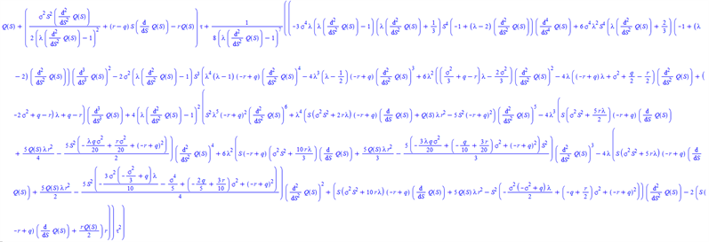
Maple generated the fourth degree symbolic approximate for $V\left(S,\tau \right)$ with $V\left(S,0\right)=Q_3\left(S\right)$ but the output was too large to present but the coefficient of $\tau$ is

To emphasize, note that Maple can be used to generate the Greeks symbolically and then these can be analyzed in a variety of ways. Of course, as pointed out in this paper and the linear paper, all the Greeks can be generated numerically using the discrete PSM J polynomials approximating $V\left(S,\tau \right)$ at $S_i$.

Conflicts of Interest

The authors declare no conflicts of interest.

References

[1]	Buetow, G. and Sochacki, J. (2019) Introducing the Power Series Method to Numerically Approximate Contingent Claim Partial Differential Equations. Journal of Mathematical Finance, 9, 616-636. https://doi.org/10.4236/jmf.2019.94031
[2]	Leland, H. (1985) Option Pricing and Replication with Transactions Costs. The Journal of Finance, 40, 1283-1301. https://doi.org/10.1111/j.1540-6261.1985.tb02383.x
[3]	Merton, R. (1973) Theory of Rational Option Pricing. The Bell Journal of Economics and Management Science, 4, 141-183. https://doi.org/10.2307/3003143
[4]	Black, F. and Scholes, M. (1973) The Pricing of Options and Corporate Liabilities. The Journal of Political Economy, 81, 637-654. https://doi.org/10.1086/260062
[5]	Parker, G. and Sochacki, J. (1996) Implementing the Picard Iteration. Neural, Parallel, and Scientific Computations, 4, 97-112.
[6]	Parker, G. and Sochacki, J. (2000) A Picard-McLaurin Theorem for Initial Value PDE’s. Abstract Analysis and Its Applications, 5, 47-63. https://doi.org/10.1155/S1085337500000063
[7]	Amster, P. and Mogni, A.P. (2018) Adapting the CVA Model to Leland’s Framework.
[8]	Amster, P., Averbuj, C.G., Mariani, M.C. and Rial, D. (2005) A Black-Scholes Option Pricing Model with Transaction Costs. Journal of Mathematical Analysis and Applications, 303, 688-695. https://doi.org/10.1016/j.jmaa.2004.08.067
[9]	Bakstein, D. and Howison, S. (2003) A Non-Arbitrage Liquidity Model with Observable Parameters for Derivatives. Working Paper, Oxford Centre for Industrial and Applied Mathematics, Oxford, 1-52.
[10]	Barles, G. and Soner, H.M. (1998) Option Pricing with Transaction Costs and a Nonlinear Black-Scholes Equation. Finance and Stochastics, 2, 369-397. https://doi.org/10.1007/s007800050046
[11]	Boyle, P. and Vorst, T. (1992) Option Replication in Discrete Time with Transaction Costs. The Journal of Finance, 47, 271-293. https://doi.org/10.1111/j.1540-6261.1992.tb03986.x
[12]	Ehrhardt, M. (2008) Nonlinear Models in Mathematical Finance: New Research Trends in Option Pricing. Nova Science Publishers, New York.
[13]	Frey, R. (1998) Perfect Option Replication for a Large Trader. Finance and Stochastics, 2, 115-142. https://doi.org/10.1007/s007800050035
[14]	Frey, R. and Patie, P. (2002) Risk Management for Derivatives in Illiquid Markets: A Simulation Study. In: Sandmann, K. and Schönbucher, P.J., Eds., Advances in Finance and Stochastics: Essays in Honour of Dieter Sondermann, Springer, Berlin, 137-159. https://doi.org/10.1007/978-3-662-04790-3_8
[15]	Frey, R. and Stremme, A. (1997) Market Volatility and Feedback Effects from Dynamic Hedging. Mathematical Finance, 7, 351-374. https://doi.org/10.1111/1467-9965.00036
[16]	Wilmott, P. (2000) Paul Wilmott on Quantitative Finance (Vol. I, II). Wiley, New York.
[17]	Hoggard, T., Whaley, A. and Wilmott, P. (1994) Hedging Option Portfolios in the Presence of Transaction Costs. Advances in Futures and Options Research, 7, 21-35.
[18]	Schonbucher and Wilmott (2000) The Feedback Effect of Hedging in Illiquid Markets. SIAM Journal of Applied Mathematics, 61, 232-272. https://doi.org/10.1137/S0036139996308534
[19]	Frey, R. (2000) Market Illiquidity as a Source of Model Risk in Dynamic Hedging. In: Gibson, R., Ed., Model Risk, Risk Publications, London, 125-136.
[20]	Liu, H. and Yong, J. (2005) Option Pricing with an Illiquid Underlying Asset Market. Journal of Economic Dynamics and Control, 29, 2125-2156. https://doi.org/10.1016/j.jedc.2004.11.004
[21]	Abe, R. and Ishimura, N. (2008) Existence of Solutions for the Nonlinear Partial Differential Equation Arising in the Optimal Investment Problem. Proceedings of the Japan Academy Series A, 84, 11-14. https://doi.org/10.3792/pjaa.84.11
[22]	Ankudinova, J. and Ehrhardt, M. (2008) On the Numerical Solution of Nonlinear Black-Scholes Equations. Computers & Mathematics with Applications, 56, 799-812. https://doi.org/10.1016/j.camwa.2008.02.005
[23]	Anwar, M. and Andallah, L. (2018) A Study on Numerical Solution of Black-Scholes Model. Journal of Mathematical Finance, 8, 372-381. https://doi.org/10.4236/jmf.2018.82024
[24]	Arenas, A.J., Gonzalez-Parra, G. and Caraballo, B.M. (2013) A Nonstandard Finite Difference Scheme for a Nonlinear Black-Scholes Equation. Mathematical and Computer Modelling, 57, 1663-1670. https://doi.org/10.1016/j.mcm.2011.11.009
[25]	Cen, Z. and Le, A. (2011) A Robust and Accurate Finite Difference Method for a Generalized Black-Scholes Equation. Journal of Computational and Applied Mathematics, 235, 3728-3733. https://doi.org/10.1016/j.cam.2011.01.018
[26]	Company, R., Jodar, L. and Pintos, J.R. (2009) A Numerical Method for European Option Pricing with Transaction Costs Nonlinear Equation. Mathematical and Computer Modelling, 50, 910-920. https://doi.org/10.1016/j.mcm.2009.05.019
[27]	Cont, R. and Voltchkova, E. (2005) A Finite Difference Scheme for Option Pricing in Jump Diffusion and Exponential Levy Models. Journal on Numerical Analysis, 43, 1596-1626. https://doi.org/10.1137/S0036142903436186
[28]	Duffie, D. (2006) Finite Difference Methods in Financial Engineering: A Partial Differential Equation Approach. John Willy & Sons, Hoboken. https://doi.org/10.1002/9781118673447
[29]	Forsyth, P. and Labahn, G. (2007) Numerical Methods for Controlled Hamilton-Jacobi-Bellman PDEs in Finance. Journal of Computational Finance, 11, 1-44. https://doi.org/10.21314/JCF.2007.163
[30]	Giles, M. and Carter, R. (2006) Convergence Analysis of Crank-Nicolson and Rannacher Time-Marching. Journal of Computational Finance, 9, 89-112. https://doi.org/10.21314/JCF.2006.152
[31]	Gonzalez-Parra, G., Arenas, A. and Chen-Charpentier, B. (2014) Positive Numerical Solution for a Nonarbitrage Liquidity Model Using Nonstandard Finite Difference Schemes. Numerical Methods for Partial Differential Equations, 30, 210-221. https://doi.org/10.1002/num.21804
[32]	Jandacka, M. and Sevcovic, D. (2005) On the Risk-Adjusted Pricing-Methodology-Based Valuation of Vanilla Options and Explanation of the Volatility Smile. Journal of Applied Mathematics, 3, 235-258. https://doi.org/10.1155/JAM.2005.235
[33]	Koleva, M.N. and Vulkov, L.G. (2017) Computation of Delta Greek for Non-Linear Models in Mathematical Finance. In: Dimov, I., Farago, I. and Vulkov, L., Eds., Numerical Analysis and Its Applications, Lecture Notes in Computer Science, Volume 10187, Springer, Berlin, 430-438. https://doi.org/10.1007/978-3-319-57099-0_48
[34]	Kutik, P. and Mikula, K. (2011) Finite Volume Schemes for Solving Nonlinear Partial Differential Equations in Financial Mathematics. In: Fort, J., et al., Eds., Finite Volumes for Complex Applications VI and Perspectives, Springer, Berlin, 643-651. https://doi.org/10.1007/978-3-642-20671-9_68
[35]	Lesmana, D. and Wang, S. (2013) An Upwind Finite Difference Method for a Nonlinear Black-Scholes Equation Governing European Option Valuation under Transaction Costs. Applied Mathematics and Computation, 219, 8811-8828. https://doi.org/10.1016/j.amc.2012.12.077
[36]	Sevcovic, D. (2017) Nonlinear Parabolic Equations Arising in Mathematical Finance. In: Ehrhardt, M., et al., Eds., Novel Methods in Computational Finance, Vol. 25, Springer, Berlin, 3-15. https://doi.org/10.1007/978-3-319-61282-9_1
[37]	Sevcovic, D., Stehlikova, B. and Mikula, K. (2011) Analytical and Numerical Methods for Pricing Financial Derivatives. Nova Science Publishers, Inc., Hauppauge.
[38]	Sevcovic, D. and Zitnanska, M. (2016) Analysis of the Nonlinear Option Pricing Model under Variable Transaction Costs. Asia-Pacific Financial Markets, 23, 153-174. https://doi.org/10.1007/s10690-016-9213-y
[39]	Wang, J. and Forsyth, P. (2008) Maximal Use of Central Differencing for Hamilton-Bellman PDE’s in Finance. SIAM Journal of Numerical Analysis, 46, 1580-1601. https://doi.org/10.1137/060675186
[40]	Zhou, S., Han, L., Li, W., Zhang, Y. and Han, M. (2015) A Positivity-Preserving Numerical Scheme for Option Pricing Model with Transaction Costs under Jump-Diffusion Process. Computational and Applied Mathematics, 34, 881-900. https://doi.org/10.1007/s40314-014-0156-5
[41]	Zhou, S., Li, W., Wei, Y. and Wen, C. (2012) A Positivity-Preserving Numerical Scheme for Nonlinear Option Pricing Models. Journal of Applied Mathematics, 2012, Article ID: 205686. https://doi.org/10.1155/2012/205686
[42]	Brennan, M. and Schwartz, E. (1978) Finite Difference Methods and Jump Processes Arising in the Pricing of Contingent Claims: A Synthesis. Journal of Financial and Quantitative Analysis, 13, 461-474. https://doi.org/10.2307/2330152
[43]	Buetow, G. and Sochacki, J. (1995) A Finite Difference Approach to the Pricing of Options Using Absorbing Boundary Conditions. Journal of Financial Engineering, 4, 263-280.
[44]	Buetow, G. and Sochacki, J. (1998) A More Accurate Finite Difference Approach to the Pricing of Contingent Claims. Applied Mathematics and Computation, 91, 111-126. https://doi.org/10.1016/S0096-3003(97)10029-7
[45]	Buetow, G. and Sochacki, J. (2000) The Tradeoffs Between Alternative Finite Difference Techniques Used to Price Derivative Securities. Applied Mathematics and Computation, 115, 177-190. https://doi.org/10.1016/S0096-3003(99)00141-1
[46]	Frey, R. and Polte, U. (2010) NonlinEAR Black-Scholes Equations in Finance: Associated Control Problems and Properties of Solutions. SIAM Journal Control Optimization, 49, 185-204. https://doi.org/10.1137/090773647
[47]	Matic, I., Radoicic, R. and Stefanica, D. (2020) A PDE Method for Estimation of Implied Volatility. Quantitative Finance, 20, 393-408. https://doi.org/10.1080/14697688.2019.1675898
[48]	Glover, K., Duck, P. and Newton, D. (2010) On Nonlinear Models of Markets with Finite Liquidity: Some Cautionary Notes. SIAM Journal of Applied Mathematics, 70, 3252-3271. https://doi.org/10.1137/080736119
[49]	Kyle, A. (1985) Continuous Auctions and Insider Trading. Econometrica, 53, 1315-1335. https://doi.org/10.2307/1913210
[50]	Hoffman, J.D. and Frankel, S. (2018) Numerical Methods for Engineers and Scientists. United States: CRC Press, Boca Raton. https://doi.org/10.1201/9781315274508
[51]	Evans, G.A., Blackledge, J.M. and Yardley, P.D. (2000) Numerical Methods for Partial Differential Equations. Springer, Berlin. https://doi.org/10.1007/978-1-4471-0377-6
[52]	Money, J. (2006) Variational Methods for Image Deblurring and Discretized Picard’s Method. Ph.D. Thesis, University of Kentucky, Kentucky.
[53]	Sochacki, J.S. (2010) Polynomial Ordinary Differential Equations—Examples, Solutions, Properties. Neural Parallel & Scientific Computations, 18, 441-450.
[54]	Heider, P. (2010) Numerical Methods for Non-Linear Black-Scholes Equations. Applied Mathematical Finance, 17, 59-81. https://doi.org/10.1080/13504860903075670