1. Introduction: Reducing Transformations Applied to Global Optimization
This paper is concerned with computational resolution of a Boolean Equation of 21 variables. In this paper, it proposes new reducing transformations allowing us to simplify a multivariable optimization problem to a new optimization problem according to a single variable. The Alienor method has been elaborated at the beginning of the 1980s by Yves Cherruault and Arthur Guillez (1983). The following people have also greatly contributed to the improvement of this new optimization method: Blaise Somé, Gaspar Mora, Balira Konfé, Jean Claude Mazza and Esther Claudine Bityé Mvondo. Let us recall the definition of an alpha-dense curve [2] [3].
1.1. Definition
A subspace
of a compact
is said α-dense, if for any point
, there exists
such that the Euclidian distance d satisfies
. In other words, we can approach any
by a point of
to within α.
Our new method is described as follows. Let
(1)
be a reducing transformation, α-dense curve in a compact set of
and f a continuous function satisfying the condition
(2)
with this method the global minimization problem
(3)
becomes
(4)
by using the α-dense curve
(5)
where
(6)
The global minimum of
has to be found in an interval
where
is bounded and independent of n. An approximation of this global minimum is obtained by choosing a step
and by discretizing the bounded interval
by means of the points
where i is an integer,
with
. The discretized problem associated to our problem is therefore
(7)
when
, equation
(8)
leads to approximations of
(9)
1.2. Theorem
Every (local or global) minimum of
can be approximated by a minimum of
.
Proof
Let
be a point realizing a minimum of f. Let
be a point on the α-dense curve minimizing the distance between
and
Furthermore, let
be the point ensuring the minimum of
.
Recall that
is the restriction of f to the α-dense curve defined by
(5)
We have the following inequality
Because
is a restriction of f to a subset of
.
But f is continuous and
tends to
when the density parameter α tends to 0. Then we have
involving:
with
, arbitrary small.
Moreover, we have
involving
We deduce
Consequently,
tends to
when α tends to 0.
Suppose that
does not tend to
. The continuity of f implies that there exists
(
does not tend to 0) such that
But we have
This contradiction proves the result.
1.3. Remark
If
(5)
is a reducing transformation for real numbers then,
(10)
is a reducing transformation for positive real numbers,
(11)
or
(12)
are reducing transformations for positive integer numbers, and
(13)
is a reducing transformation for binary numbers.
Where ABS is the absolute value; INT is the integer part; MOD is the modulo function;
varies from 0 to
;
is a positive integer number. We can use the function INT or round.
We will carry out the necessary demonstrations in the next papers. The main idea of our method consists in expressing n variables by means of a single variable. The Alpha-dense Curves generalize the Space-filling Curves. We have used the properties of the Archimedean Spiral to build reducing transformations.
1.4. The Archimedean Spiral
1.4.1. Dimension 2
Let us draw this example of the Archimedean Spiral (Figure 1).
1.4.2. Dimension 3
So we have
It results
1.4.3. Dimension 4
Then
We use the following reducing transformations.
1.5. Reducing Transformations
1.5.1. For Real Numbers
(14)
(15)
(16)
(17)
(18)
(19)
(20)
(21)
(22)
(23)
Some curves
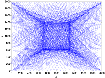
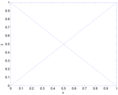
Let us consider this reducing transformation
For instance, let us draw the curve
We obtain the curve below by setting with Matlab
close all;
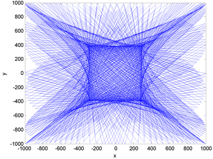
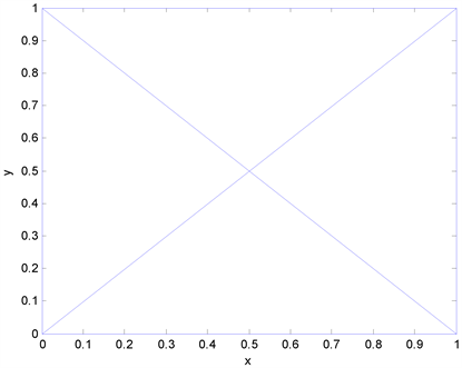
And for
For instance, let us draw the curve
We obtain the curve below by setting with Matlab
close all;
1.5.2. For Positive Real Numbers
(24)
(25)
(26)
(27)
(28)
(29)
(30)
(31)
(32)
(33)
1.5.3. For Positive Integer Numbers
(34)
(35)
(36)
(37)
(38)
(39)
(40)
(41)
(42)
(43)
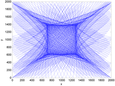
Let us consider this reducing transformation
For instance, let us draw the curve
We obtain the curve below by setting with Matlab
close all;
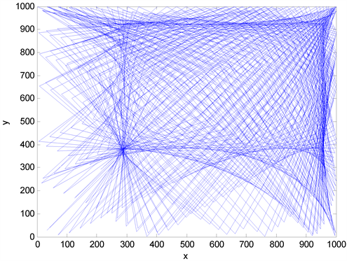
And for
For instance, let us draw the curve
We obtain the curve below by setting with Matlab
close all;
We also have these reducing transformations:
(44)
(45)
(46)
(47)
(48)
(49)
(50)
(51)
(52)
(53)
For binary numbers
(54)
(55)
(56)
(57)
(58)
(59)
(60)
(61)
(62)
(63)
Let us consider this reducing transformation
For instance, let us draw the curve
We obtain the curve below by setting with Matlab
close all;
And for
For instance, let us draw the curve
We obtain the curve below by setting with Matlab
close all;
where ABS is the absolute value; INT is the integer part (we can also use the function round); MOD is the modulo function;
is a real number,
,
and K are prime numbers; T varies from 0 to
;
is a positive integer number.
2. Applications
We can use different softwares like Microsoft Excel, Maple or others, to program this method.
2.1. With Excel
Excel is a software developed at the beginning of 1980s by Microsoft. The Excel tabulator helps to create spreadsheets, to view, to edit and share them with others quickly and easily.
2.1.1. Reducing Transformations
We use the following reducing transformations.
1) For real numbers
2) For positive real numbers
3) For positive integer numbers
4) For binary numbers
where ABS is the absolute value; INT is the integer part (we can also use the function round); MOD is the modulo function;
is a real number,
,
and K are prime numbers; T varies from 0 to
;
is a positive integer number and
is the sign “multiply by”.
2.1.2. Application
With Excel, we have the following table
with this powerful technique, we can solve:
● Boolean Equations.
● Diophantine Equations.
● 0 - 1 integer programming problems.
● Mixed integer programming problems.
● Integer programming problems.
● Partial Differential Equations.
● Etc.
2.1.3. Examples
Let us look at some examples.
1) Resolution of a Boolean Equation of 3 variables and 21 variables
Boolean Algebra is a deductive mathematical system closed over the values 0 and 1 (false and true). Boolean Logic forms the basis for computation in modern binary computer systems. We can represent any electronic computer circuit by using a system of Boolean Equations. We usually represent Boolean Functions by means of truth tables. A statement with n logical variables requires a table with 2n rows.
a) Resolution of a Boolean Equation of 3 variables
Let us solve [1]
We set
We calculate
T from 0 to 6.5514 step 0.0001
And we have four solutions, the first solution
is first obtained when
;
The second solution
is first obtained when
;
The third solution
is first obtained when
;
And the fourth solution
is first obtained when
.
We obtain the following table
It is easy to represent the truth table, because we have 23 (8) rows. The truth table is given below.
b) Resolution of a Boolean Equation of 21 variables
For twenty one variables, it is difficult to represent the truth table (221 = 2,097,152 rows).
Let us solve
We set
We calculate
T from 0 to 6.5514 step 0.0001
And we have 11,192 solutions, the first solution
is obtained when
;
The second solution
is obtained when
;
The third solution
is obtained when
;
The fourth solution
is obtained when
;
The fifth solution
is obtained when
;
The sixth solution
is obtained when
;
…
The before last solution
is obtained when
;
The last solution
is obtained when
.
2) Resolution of a Diophantine Equation
Let us solve the system
We set
T from 0 to 6.5514 step 0.0001
We calculate
We obtain the following table
And we find
when
.
3) Resolution of a 0 - 1 integer programming problem
Let us maximize
Subject to
We set
T from 0 to 6.5514 step 0.0001
We obtain the following table
And we find
when
.
4) Resolution of a mixed integer programming problem
Let us minimize
Subject to
a real;
and
are integers;
We set
T from 0 to 6.5514 step 0.0001
We obtain the following table
And we find
when
.
5) Resolution of an integer programming problem
Let us maximize
Subject to
and
are integers;
We set
T from 0 to 6.5514 step 0.0001
We obtain the following table
And we find
when
.
3. Conclusion
This article is the continuation of two previous papers: Computational resolution of Diophantine Equations by means of Alpha-dense Curves (2012) and Global Optimization with Alpha-dense Curves: resolution of Boolean Equations (2012) from Esther Claudine Bityé Mvondo, Yves Cherruault, and Jean Claude Mazza. We have proposed new reducing transformations allowing us to simplify a multivariable optimization problem to a new optimization problem according to a single variable. We have shown, in different examples, how to use Alpha-dense Curves to solve different Mathematical Programming problems by means of the tabulator Microsoft Excel such as a Boolean Equation of three variables, and a Boolean Equation of twenty-one variables. We will carry out the necessary demonstrations in the next papers. Differential Equations and Partial Differential Equations can also be solved with this powerful technique. We can also easily solve problems involving a large number of variables with the tabulator Excel of Microsoft. We can use different softwares like Microsoft Excel, Maple or others, to program our method.
Dedicated
This paper is dedicated to my ALMIGHTY FATHER.