An Improved Time Series Symbolic Representation Based on Multiple Features and Vector Frequency Difference

Lijuan Yan^*, Xiaotao Wu, Jiaqing Xiao

College of Mathematics and Statistics, Huanggang Normal University, Huanggang, China.

DOI: 10.4236/jcc.2022.106005                

Abstract

Symbolic Aggregate approXimation (SAX) is an efficient symbolic representation method that has been widely used in time series data mining. Its major limitation is that it relies exclusively on the mean values of segmented time series to derive the symbols. So, many important features of time series are not considered, such as extreme value, trend, fluctuation and so on. To solve this issue, we propose in this paper an improved Symbolic Aggregate approXimation based on multiple features and Vector Frequency Difference (SAX_VFD). SAX_VFD discriminates between time series by adopting an adaptive feature selection method. Furthermore, SAX_VFD is endowed with a new distance that takes into account the vector frequency difference between the symbolic sequence. We demonstrate the utility of the SAX_VFD on the time series classification task. The experimental results show that the proposed method has a better performance in terms of accuracy and dimensionality reduction compared to the so far published SAX based reduction techniques.

Keywords

Time Series, Representation, SAX, Feature Selection, Classification

1. Introduction

A time series is a sequence of observations taken sequentially in time [1]. The data in most application fields in the real world are stored in the form of time series data. Meteorological data in weather forecast, foreign trade floating exchange rate, radio waves, images collected by medical devices, continuous signals in engineering applications, biometric data (image data of face recognition), particle tracking in physics, etc. These data can be processed as time series. With the continuous innovation and application of Internet of things, cloud computing, next generation mobile communication and other information technologies, the amount of time series data increases exponentially. Time series data mining has attracted enormous attention in the last decade [2] [3] [4].

The most obvious nature of time series includes large in data size and high dimensionality. Data mining directly from the original series is not only time-consuming but also inefficient. Therefore, in the context of time series data mining, the fundamental problem is how to represent the time series data [5]. Time series representation is a common dimension reduction technology in time series data mining. It represents the original time series in another space through transformation or feature extraction. It can reduce the data to manageable size and retain the important characteristics of the original data. In recent years, time series representation has arisen as a relevant research topic. A great number of time series representations have been introduced. The techniques of time series representation are divided into two main categories: data adaptive such as Adaptive Piecewise Constant Approximation (APCA) [6], and non-data adaptive such as Discrete Fourier Transform (DFT) [7] [8] [9]. Each method aims to support similarity search and data mining tasks, and most of them [10] - [16] focus on data compression efficiency.

Symbolic Aggregate approXimation (SAX) is a data adaptive technique that transforms a time series into a symbolic sequence [16]. SAX is the first symbolic representation method to reduce and index dimensions by using the boundary distance measure which is lower than Euclidean distance [10] [17]. In the classic time series mining tasks, such as classification, clustering, indexing, SAX can achieve the similar performance as other famous methods such as Discrete Wavelet Transform (DWT) [11] and Discrete Fourier Transform (DFT) [18], but it only needs less storage space. In addition, this discrete feature representation method enables researchers to use the rich data structures and algorithms in text mining to solve various tasks of time series data mining, which has great expansion and application potential.

The SAX’s major limitation is that it extracts exclusively the mean feature of segmented time series to derive the symbols. However, many important features of time series are not considered, such as extreme value, trend, fluctuation and so on. Different segments with similar mean values may be mapped to the same symbols. It does not distinguish the segments with similar mean values very well.

There have been some improvements of the SAX representation which focus on the selection of extracted features. Some methods improve the SAX by replacing mean feature with trend feature. SAX-TD [19] uses the starting and the ending points of segment approximatively determine a trend and proposes a modified distance accordingly. SAX-DR [20] encodes the direction of segment as trend feature. Each time series segment is mapped to one of the three directions: convex, concave and linear. SAX-CP [21] captures the trend through the assessment of variation between a point and a segment mean. Some methods improve the SAX by increasing the number of extracted features. For example, ESAX [22] extracts three features for each segment, the original mean value and additional min and max value, which are used for time series data representation. ESAX triples the storage cost with respect to the original SAX representation but enjoys better classification accuracy results than the SAX. SFVS [23] utilizes a symbolic representation based on the summary of statistics of segment. It considers the symbols as a vector, including the mean and variance feature as two elements. These research results also have shown that it is very important to extract appropriate features for discretization. According to the characteristics of different types of data sets, how to extract appropriate features is a problem worthy of discussion.

We propose in this paper an improved Symbolic Aggregate approXimation based on multiple features and Vector Frequency Difference (SAX_VFD). Three main contributions have been made in this work. Firstly, an adaptive feature selection method is proposed to optimize the insufficient representation of single feature. Each time series segment is transformed into a vector that includes four selected feather values of that segment. Secondly, a new distance that takes into account the vector frequency difference between the symbolic sequence is introduced. Our improved distance measure keeps a lower-bound to the Euclidean distance. Thirdly, a comprehensive set of experiments, which shows the benefits of using SAX_VFD in enhancing the accuracy of time series classification, has been conducted.

The rest of this paper is organized as follows. Section 2 provides the background knowledge of SAX. Section 3 introduces our SAX_VFD technique. Section 4 contains an experimental evaluation on several time series data sets. Finally, Section 5 offers some conclusion and suggestions for future work.

2. Symbolic Aggregate ApproXimation (SAX)

The SAX mainly includes three steps. Firstly, each time series is normalized to have a mean of zero and a standard deviation of one, since it is convenient for comparing time series with different offsets and amplitudes [2].

Secondly, Piecewise Aggregate Approximation (PAA) [24] is used to transform a time series into equally sized segments. In short, PAA is to divide the time series into equal size segments, and use the average value of each segment as a simplified representation of the original data. A time series $C=\langle c_1,c_2,c_3,\cdots ,c_n\rangle$ of length n can be represented in a ω-dimensional space by a vector $\bar{C}=\langle {\bar{c}}_1,{\bar{c}}_2,{\bar{c}}_3,\cdots ,{\bar{c}}_{\omega }\rangle$. The th element of $\bar{C}$ is calculated by the following Equation (1):

${\bar{c}}_i=\frac{\omega }{n}{\displaystyle {\sum }_{j=\frac{n}{\omega }\left(i-1\right)+1}^{\frac{n}{\omega }i}{c}_j}$ (1)

Finally, the PAA transformed features are applied a further transformation to obtain a word based on the breakpoints interval it falls in. Given that the normalized time series have highly Gaussian distribution, the breakpoints can divide the area under distribution into α equiprobable regions where α is the alphabet size. A lookup table that contains the breakpoints is shown in Table 1.

The features transformed from PAA can be mapped to specific alphabet symbol according to the results of Table 1. If the feature falls in the interval $\left(-\infty ,{\beta }_1\right)$, it is mapped to the alphabet symbol “A”. If the feature falls in the interval $\left[{\beta }_2,{\beta }_3\right)$, it is mapped to the alphabet symbol “B” and so on. As shown in Figure 1, a time series of length 470 is mapped to the word “DDDEA”, where the number of segments ω is 5 and the size of alphabet α is 6. Through the SAX transformation, a time series of length n obtain a discrete and symbolic representation $\hat{C}=\langle {\hat{c}}_1,{\hat{c}}_2,{\hat{c}}_3,\cdots ,{\hat{c}}_{\omega }\rangle$.

For the utilization of the SAX in classic data mining tasks, the distance called MINDIST was proposed. Given two time series Q and C with the same length n, $\hat{Q}$ and $\hat{C}$ are their SAX representation with the number of segments ω, the distance MINDIST between these two symbolic sequences is defined in Equation (2).

Figure 1. A time series of length 470 is mapped to the word “DDDEA”, where ω is 5 and α is 6.

Table 1. A lookup table for breakpoints with the alphabet size from 3 to 10.

$MINDIST\left(\hat{Q},\hat{C}\right)=\sqrt{\frac{n}{\omega }}\sqrt{{\displaystyle {\sum }_{i=1}^{\omega }{\left(dist\left({\hat{Q}}_i,{\hat{C}}_i\right)\right)}^2}}$ (2)

where the dist() function can be implemented using Table 1, and is calculated by Equation (3).

$dist\left({\hat{Q}}_i,{\hat{C}}_i\right)=\{\begin{array}{l}0,\text{if}\left|{\hat{Q}}_i-{\hat{C}}_i\right|\le 1\\ {\beta }_{\max \left({\hat{Q}}_i,{\hat{C}}_i\right)-1}-{\beta }_{\min \left({\hat{Q}}_i,{\hat{C}}_i\right)},\text{otherwise}\end{array}$ (3)

The SAX representation can approximately represent the original time series, where the parameter ω controls the number of approximation and the parameter α controls the granularity of approximate symbols. The choice of parameters is highly dependent on data.

3. Proposed Technique

As we reviewed at Section 1, using the SAX the time series can be mapped to symbols by the mean feature of segments. But this representation is imprecise due to differences between data sets. For financial data, volatility and extreme value are important features, while for meteorological data, more attention is paid to the trend and periodicity of data. Therefore, for different datasets, extracting the same features is not conducive to distinguish time series.

In this paper, we use a feature vector to represent each segment of time series. The elements in the vector depend on the result of feature selection. To go a step further, we introduce a new distance measurement method, which takes the vector frequency difference as the weight of different feature distances based on the classic SAX.

3.1. Optimal Feature Vector

After dimensionality reduction of the original time series, if the distance between two points in the original space is less than the threshold, but the distance between the two points in the reduced feature space is greater than the threshold, the false dismissals will be caused.

Faloutsos et al. introduced lower bounding [18]. It is proved that in order to guarantee no false dismissals, the distance measure in the reduced feature space must satisfy the condition as described in Equation (4).

$D_{feature}\left(F\left(O_1\right),F\left(O_2\right)\right)\le D_{object}\left(O_1,O_2\right)$ (4)

where $O_1$ and $O_2$ are the two objects in original space, their distance is $D_{object}\left(\right)$ ; $F\left(O_1\right)$ and $F\left(O_2\right)$ are the feature extracting function, the distance in reduced feature space.

To assess the distance quality, the Tightness of Lower Bound (TLB) [2] metric is used. TLB is defined as Equation (5).

$\text{TLB}=\frac{\text{lower bound distance}}{\text{true euclidean distance}}$ (5)

The value of TLB is between 0 and 1. The closer to 1 is this fraction, the better is the TLB, which shows that the distance after dimensionality reduction is closer to the original distance.

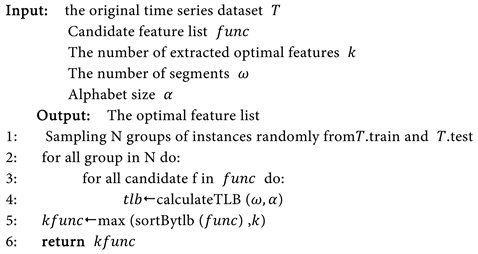
Based on this point, we propose an optimal feature vector selection algorithm. For a specific data set, the features which have larger TLB value are selected. Algorithm 1 describes the process of optimizing feature vector.

Firstly, N groups of samples are randomly selected from the training set and the test set. The candidate feature quantity is calculated, and the distance between words is calculated using the classic SAX. Divided by the Euclidean distance between the original samples to get the value of tlb. According to the definition of TLB, the closer to 1 is this fraction, the better is the TLB. Therefore, we keep the k features with the largest tlb mean value as the optimal features. In this paper, the value of N is one tenth of the length of the training set. If the length of the training set is less than 50, the value of n is half of the length of the training set to ensure the stability of the selected features. The k value is set to 4.

From the perspective of pattern recognition [25], it is more efficient to characterize time series using some key classes of methods, including autocorrelation, stationarity, entropy, and methods from the physics-based nonlinear time series analysis [26]. For the candidate feature list func, we refers to the feature extraction method in tsfresh [27] module. SAX_VFD proposed in this paper provides a total of 18 features in three categories: statistical features, entropy features and fluctuation features.

1) Statistical features

There are 9 statistical features, including maximum (max), minimum (min) and mean (μ), median (median), variance (σ²), skewness (SKEW), kurtosis (KURT), range (R) and interquartile range (IQR). $X_n=\langle x_1,x_2,x_3,\cdots ,x_n\rangle$ is a time series of length n, the statistical features are calculated by Equations as follows:

$\mu =\frac{1}{n}{\displaystyle {\sum }_{i=1}^n{x}_i}$ (6)

${\sigma }^2={\displaystyle {\sum }_{i=1}^n\frac{1}{n}{\left(x_i-\mu \right)}^2}$ (7)

Algorithm 1. Feature vector selection (T, func, k, ω, α).

$SKEW\left(X\right)=\frac{1}{n}{\displaystyle {\sum }_{i=1}^n\frac{{\left(x_i-\mu \right)}^3}{{\sigma }^3}}$ (8)

$KURT\left(X\right)=\frac{1}{n}{\displaystyle {\sum }_{i=1}^n\frac{{\left(x_i-\mu \right)}^4}{{\sigma }^4}}-3$ (9)

$R=\max \left(X_n\right)-\min \left(X_n\right)$ (10)

$IQR=Q_3-Q_1$ (11)

2) Entropy features

Usually, the statistical characteristics alone cannot accurately distinguish time series very well. Entropy can be used to describe the uncertainty and complexity of time series. In this paper, four kinds of entropy features of time series are adopted, which are entropy, binned entropy, approximate entropy and sample entropy.

According to the concept of information entropy in information theory, the more orderly a system is, the lower its information entropy is. The more chaotic a system is, the higher its information entropy is. Information entropy is a measure of the degree of system ordering, so it can describe the randomness of time series to a certain extent. Information entropy is calculated by Equation (12).

$entropy\left(X\right)=-{\displaystyle \underset{i=1}{\overset{\infty }{\sum }}P\left\{x=x_i\right\}\ln \left(P\left(x=x_i\right)\right)}$ (12)

First bins the values of X_n into maxbin equidistant bins, then the binned entropy (bEn) is calculated by Equation (13).

$bEn\left(X\right)=-{\displaystyle {\sum }_{KE=0}^{\min \left(maxbin,len\left(X\right)\right)}{P}_k\ln \left(P_k\right)\cdot 1_{\left(P_k>0\right)}}$ (13)

where P_k is the percentage of samples in bin k, maxbin is the maximal number of bins, len(X) is the length of X.

If the bEn is large, it means that the values of this time series are evenly distributed in the range of min(X_n) and max(X_n). If the bEn is small, it means that the value of the time series is concentrated in a certain segment.

Approximate entropy (apEn) and sample entropy (sampEn) are created to measure the repeatability or predictability within a time series. Both features are extremely sensitive to their input parameters: m (the length of the compare window) and r (the similar tolerance border) and n (length of time series).

Approximate entropy is defined as the conditional probability to maintain its similarity when the similarity vector increases from m to m + 1 in dimension as described in Equation (14). The physical meaning is the probability of generating new patterns in a time series when the dimension changes. The more the probability to generate new patterns, the more complex the sequence becomes, and the larger the apEn. In theory, the apEn can reflect the degree and length of the numerical variation.

$apEn\left(X\right)={\Phi }_m\left(r\right)-{\Phi }_{m+1}\left(r\right)$ (14)

The $C_i^m\left(r\right)$ values measure the regularity within a tolerance r, or the frequency of patterns similar to a given pattern of the window length m. ${\Phi }_m\left(r\right)$ is the average value of $\ln \left(C_i^m\left(r\right)\right)$, where ln is the natural logarithm.

${\Phi }_m\left(r\right)=\frac{{\displaystyle {\sum }_{i=1}^{N-m+1}\ln \left(C_i^m\left(r\right)\right)}}{N-m+1}$ (15)

The calculation process of sample entropy is similar to that of approximate entropy. The natural logarithm is not used to calculate the average similarity rate.

$B_m\left(r\right)=\frac{{\displaystyle {\sum }_{i=1}^{N-m+1}{C}_i^m\left(r\right)}}{N-m+1}$ (16)

But the natural logarithm is used to calculate the sample entropy.

$sampEn\left(X\right)=-\ln \left[\frac{B_{m+1}\left(r\right)}{B_m\left(r\right)}\right]$ (17)

The smaller the sample entropy is, the stronger the autocorrelation is. In this paper, we utilize the recommended parameter values. The parameter m is set to 3, r is set to 0.2 times the standard deviation of the original sequence.

3) Fluctuation features

In addition, there are five features to characterize the fluctuation of time series. They are slope (slope), absolute energy (abs_energy), sum over first order differencing (absolute_sum_of_changes), average over first order differencing (mean_abs_changes) and the mean value of a central approximation of the second derivative (mean_second_derivative_central).

$slope=\frac{x_p-x_q}{p-q}$ (18)

Here we use the slope of the tangent between the extreme values, where x_p, x_q, p, q represent the extremum and corresponding time axis respectively.

$ab{s}_{energy}={\displaystyle {\sum }_{i=1}^n{x}_i^2}$ (19)

Absolute energy value can describe the fluctuation of the squared values of time series data.

A non-stationary time series can be converted to a stationary time series through differencing. First order differencing series is the change between consecutive data points in the series.

$absolute\text{\_}sum\text{\_}of\text{\_}changes={\displaystyle {\sum }_{i=1}^{n-1}\left|x_{i+1}-x_i\right|}$ (20)

$mean\text{\_}abs\text{\_}changes=\frac{1}{n}{\displaystyle {\sum }_{i=1,\cdots ,n-1}\left|x_{i+1}-x_i\right|}$ (21)

$mean\text{\_}second\text{\_}derivative\text{\_}central=\frac{1}{n}{\displaystyle {\sum }_{i=1,\cdots ,n-1}\frac{1}{2}\left(x_{i+2}-2\cdot x_{i+1}+x_i\right)}$ (22)

Sum over first order differencing and average over first order differencing can describe the absolute fluctuation between consecutive data points in the series. The second derivative is defined by the limit definition of the derivative of the first derivative. In definition, it represents the rate of change of first derivative, that is, the rate of change of fluctuation between consecutive data points.

3.2. Mapping Symbol Vector

The technique proposed in this paper is based on the SAX. Therefore, afterk features are selected in the previous section, in each segment, k f feature values can be calculated and mapped to k symbol characters respectively. These k symbol characters constitute a feature string vector for each segment. $V_i=\langle f_{i,1},f_{i,2},f_{i,3},\cdots ,f_{i,k}\rangle$ is the feature string vector of the ith segment. And so on, the original time series T can be represented by in a ω feature string vectors $T=\langle V_1,V_2,V_3,\cdots ,V_{\omega }\rangle$. Each element in the vector is no longer a single character, but a feature string composed of k feature values.

Taking a time series of length 470 as an example, the length of time series is 470, when the value of ω is 5, α is 6 and k is 4, the optimized feature list is max, min, median and mean. Max values and min values are respectively shown in red circles and in green Triangle, while media values are shown in yellow diamond lines and mean values are shown in brown lines in Figure 2. The characters of different colors in the figure represent they are mapped by corresponding features. Using the technique of SAX_VFD, the original time series can be represented as <“ECED”, “ECDD”, “FCDD”, “FAFE”, “EAAA”>. The length of vector is $\omega \times k=20$. The feature string vector contains multiple features, so it can better distinguish the segments. It can be observed from Figure 2, the second and third segments’ min, median and mean values are in the same probability interval, but they can still be distinguished by the max values.

3.3. Distance Measure

The extracted features are expanded from one to k, therefore, the distance measure need to be redefined. Section 2 introduces the distance measure in the

Figure 2. An example of time series represented by SAX_VFD.

SAX. Based on this, we provide a new concept named the vector frequency difference.

The idea of vector frequency comes from the concept of term frequency in text mining. Term frequency (TF) is used in connection with information retrieval and shows how frequently an expression (term, word) occurs in a document [28]. Term frequency indicates the significance of a particular term within the overall document. The famous tf-idf algorithm believes that the smaller the term frequency, the greater its ability to distinguish different types of text [29].

The distance measure is proposed in this paper based on the assumption that the smaller the frequency of a certain feature vector in the feature vector set of the whole time series data set, the greater its ability to represent time series samples. Therefore, the larger the frequency difference between the two feature string vectors, the greater the difference in the ability to distinguish samples between them, so the corresponding distance between the two should be relatively increased. According to this, the distance measure is redefined.

Given two time series Q and C with the same length n, each segmented sequence can be represented by a feature string vector, which contains k transformed characters, after K features are selected, each segmented sequence can be represented by a feature string vector, and each feature string vector contains k transformed characters. In this case, a feature string vector in Q can be represented as $V_Q=\langle {\hat{q}}_1,{\hat{q}}_2,{\hat{q}}_3,\cdots ,{\hat{q}}_k\rangle$, and a feature string vector in C can be represented as $V_C=\langle {\hat{c}}_1,{\hat{c}}_2,{\hat{c}}_3,\cdots ,{\hat{c}}_k\rangle$. The distance vdis between two feature string vectors is defined as:

$vdis\left(V_Q,V_C\right)=\sqrt{{\displaystyle {\sum }_{j=1}^k{\left(dist\left({\hat{q}}_j,{\hat{c}}_j\right)\right)}^2}}$ (23)

Each time series is composed of ω feature string vectors, $\hat{Q}$ and $\hat{C}$ are the new representation of time series of Q and C. The distance between them is defined as follows:

$DDIST\left(\hat{Q},\hat{C}\right)=\sqrt{\frac{n}{\omega }}\sqrt{\Delta vf\left(V_{Qi},V_{Ci}\right)\times {\left(vdis\left(V_{Qi},V_{Ci}\right)\right)}^2}$ (24)

where $\Delta vf\left(V_{Qi},V_{Ci}\right)$ us the frequency difference of two feature string vectors.

One of the most important features of the SAX is that it provides a lower bound distance measure. The lower bound is very useful for controlling the error rate and improving the calculation speed [2]. Because $\Delta vf\left(V_{Qi},V_{Ci}\right)<1$, the new distance measure $DDIST\left(\hat{Q},\hat{C}\right)$ proposed in this paper still satisfies the lower bound.

4. Experimental Studies

In this section we perform time series classification using SAX_VFD. Then we compare the results with the classic Euclidean distance and other preciously proposed symbolic techniques. We focus on the performance of classification error rate, dimensionality reduction and efficiency.

4.1. Experimental Dataset

In this paper, we use 24 datasets from UCR repository [30]. These have been commonly adopted by TSC researchers. The basic information of the datasets is shown in Table 2. The types of datasets used are diverse and come from several fields, including sensor data, image contour information data, device data, simulated data, etc. All data sets are of labeled, univariate time series, without any preprocessing. We used the default train and test data splits.

4.2. Experimental Design

The experiment mainly aims to confirm the proposed distance measure’s effectiveness. We do comparison experiments on the SAX_VFD with the Euclidean

Table 2. Datasets used in the experiments.

distance and other preciously proposed symbolic techniques, which are the SAX and the ESAX. To the time series classification task, distance measurement will directly affect the classification results. Therefore, we construct 1 Nearest Neighbor (1 NN) classifier based on different distance measures, and compare the error rate to observe the advantages and disadvantages of different distance measures. The advantage of this design is that the underlying distance metric is critical to the performance of 1 NN classifier, hence, the accuracy of the 1 NN classifier directly reflects the effectiveness of a distance measure. Furthermore, 1 NN classifier is parameter free, allowing direct comparisons of different measures.

Three symbolic techniques in comparative experiments, which are the SAX, the ESAX and the SAX_VFD, are impacted by the choice of the segment number ω and the alphabet size α. We try the different combination of these two parameters to test their influence on the results. For ω, we choose the value from 2 to a quarter of the length of the time series. For α, we choose the value in the range of 3 and 10.

We compare the dimension reduction effect of different techniques by the dimensionality reduction ratios when we get the best classification results. The dimensionality reduction ratio is measured as Equation (25).

$\text{Dimensionality Reduction Ratio}=\frac{\text{Number of the reduced data points}}{\text{Number of the original data points}}$ (25)

The dimensionality reduction ratio of the SAX is $\frac{\omega }{n}$, The dimensionality reduction ratio of the ESAX is $\frac{3\omega }{n}$, The dimensionality reduction ratio of the SAX_VFD is $\frac{4\omega }{n}$.

4.3. Results

The overall classification results are listed in Table 3, where entries with the lowest classification error rates are highlighted. In all 24 datasets, SAX_VFD has the lowest error in the most of the data sets (17/24), followed by the ESAX (6/24).

We use the sign test to test the significance of our proposed technique against other techniques. The sign test is a nonparametric test that can be used to test either a claim involving matched pairs of sample data.

The sign test results are displayed in Table 4, where $n_{+}$, $n_{-}$ and $n_0$ denote on the numbers of data sets where the error rates of the SAX_VFD are lower, larger than and equal to those of another technique respectively. A p-value less than or equal to 0.05 indicates a significant improvement. The smaller a p-value, the more significant the improvement. The p-values demonstrate that the distance measure of the SAX_VFD achieves a significant improvement over the other techniques on classification accuracy.

Table 3. 1 NN classification error rates of ED; 1 NN best classification error rates, ω, α and dimensionality reduction ratios of the SAX, ESAX and SAX_VFD.

Table 4. The sign test results of the SAX_VFD vs. other techniques.

To provide an illustration of the result in Table 3 more clearly, we use scatter plots for pair-wise comparisons as shown in Figure 3. In a scatter plot, the error rates of two measures under comparison are used as the x and y coordinates of a dot, where a dot represents a particular data set [31]. When a dot falls within a region, the corresponding technique in the region performs better than the other. In addition, the further a dot is from the diagonal line, the greater the margin of an accuracy improvement. The region with more dots indicates a better technique than the other.

In Figure 3, the blue dots indicate the classification error rates are lower in the upper triangle region, the red squares indicate the classification error rates are lower in the lower triangle region. In Figure 3(a), there is no obvious difference between the SAX and ED in these 24 data sets, and the number of points on both sides of the diagonal is basically the similar. In Figures 3(b)-(d), on the

(a) (b) (c) (d)

Figure 3. A pairwise comparison of classification error rates for the Euclidean distance, the SAX distance, the ESAX distance and the SAX_VFD distance. (a) SAX vs ED; (b) SAX_VFD vs ED; (c) SAX_VFD vs SAX; (d) SAX_VFD vs ESAX.

whole, our method is obviously superior to the other three techniques, both in the number of points and the distance of these points from the diagonals.

In order to understand the influence of parameter selection on the performance, we run the experiments on data sets CBF and Small Kitchen Appliances using different parameter combinations. The results are shown in Figure 4. Specially, on CBF, we firstly compare the classification error rates with different ω while α is fixed at 10, and then with different α while ω is fixed at 8; on Small Kitchen Appliances, ω varies while α is fixed at 10, and then α varies while ω is fixed at 16. The experimental results are shown in Figure 5. The SAX_VFD obtain lower classification error rates when the parameter ω are small. For example, of CBF data set, the error rate of the SAX_VFD is 0.1667 while ω is 2, it was better than the SAX (0.4122) and the ESAX (0.5). The techniques are sensitive to the parameter α. Enlarge the value of α is easy to get better classification results. Generally, the SAX_VFD can achieve better accuracy with lower parameter α. These demonstrate that the proposed technique is more significant when the parameters are small.

Totally, 447 experiments are carried out using the SAX_VFD, 1788 optimized features are adopted in these experiments. The results of feature selection are shown in Figure 5. In this divergent bar chart, the green bar on the right

(a) (b) (c) (d)

Figure 4. The classification error rates of the SAX, the ESAX and the SAX_VFD with different parameters ω and α. (a) on CBF, ω varies while α is fixed at 10; (b) on CBF, α varies while ω is fixed at 8; (c) on Small Kitchen Appliances, ω varies while α is fixed at 10; (d) on Small Kitchen Appliances, α varies while ω is fixed at 16.

represents the feature that the number of times is greater than the average value of the overall data, and the red bar on the left represents the feature that the number of times used is less than the average value of the overall data. The most frequently selected features are still the statistical features, such as mean, median, minimum and maximum. In the entropy features, the number of selected times of binned entropy is the most, and the slope is dominant in the fluctuation features.

Since one major advantage of the SAX is its dimensionality reduction, we shall compare the dimensionality reduction of the proposed technique with the SAX and the ESAX. The dimensionality reduction ratios are calculated using the parameter ω when the three techniques achieve their lowest classification error rates on each data set. The results are shown in Figure 6. The SAX_VFD is competitive with the SAX on dimensionality reduction. For each segment of time series, the SAX_VFD extract four features, it is more features than the SAX

Figure 5. The rank of feature selection times, where the average time is 99.33.

Figure 6. Dimensionality reduction ratios of the SAX, the ESAX and the SAX_VFD on 24 data sets with their lowest error rates.

and the ESAX. However, the SAX_VFD can achieve the lowest classification error rate at a smaller number of segments ω. Therefore, as shown in Figure 6, in the aspect of dimensionality reduction, the SAX_VFD is competitive with the SAX, and has advantages compared with the ESAX. For example, on CBF data set, using the SAX, when the value of ω is 32, the lowest error rate is 0.1040; while using the SAX_VFD, when the value of ω is 8, the minimum error rate is 0.0756, so the dimension reduction rate of both is 0.25.

5. Conclusions and Future Work

From the experiment, we found that although a variety of optimization features are provided, some commonly used statistical features, such as mean, median, minimum, maximum, slope, etc., can achieve good results. These statistical features are not only simple to calculate, but can better represent the time series once combined. The method proposed in this paper adds a feature representation, so it has no advantage simply from the calculation of dimension reduction

ratio. The dimensionality reduction ratio of the SAX is $\frac{\omega }{n}$, The dimensionality reduction ratio of the ESAX is $\frac{3\omega }{n}$. The dimensionality reduction ratio of the SAX_VFD is $\frac{4\omega }{n}$. However, the SAX_VFD can achieve the lowest classification

error rate at a smaller number of segments ω. While increasing the number of features, reducing the number of segments can still achieve a good effect of dimensionality reduction. From the perspective of classification error rate, the SAX_VFD has certain advantages in many data sets.

For the future work, we intend to extend the technique to other time series data mining tasks such as clustering, anomaly detection and motif discovery.

Acknowledgements

This work was supported by general topics of Hubei Educational Science Planning Project in 2021, “application of multimodality fusion analysis technology in blended learning engagement evaluation”, (NO: 2021GB069), and Doctoral Fund Project of Huanggang Normal University, (NO: 2042021020).

Conflicts of Interest

The authors declare no conflicts of interest regarding the publication of this paper.

References

[1]	Box, G.E.P., Jenkins, G.M., Reinsel, G.C. and Ljung, G.M. (2016) Time Series Analysis: Forecasting and Control. 5th Edition, John Wiley & Sons, Hoboken.
[2]	Eamonn, K. and Kasetty, S. (2003) On the Need for Time Series Data Mining Benchmarks: A Survey and Empirical Demonstration. Data Mining and Knowledge Discovery, 7, 349-371. https://doi.org/10.1023/A:1024988512476
[3]	Hasna, O.L. and Potolea, R. (2017) Time Series—A Taxonomy Based Survey. 2017 13th IEEE International Conference on Intelligent Computer Communication and Processing, Cluj-Napoca, 7-9 September 2017, 231-238. https://doi.org/10.1109/ICCP.2017.8117009
[4]	Wang, H., Zhang, Q., Wu, J., Pan, S. and Chen, Y. (2019) Time Series Feature Learning with Labeled and Unlabeled Data. Pattern Recognition, 89, 55-66. https://doi.org/10.1016/j.patcog.2018.12.026
[5]	Fu, T. (2011) A Review on Time Series Data Mining. Engineering Applications of Artificial Intelligence, 24, 164-181. https://doi.org/10.1016/j.engappai.2010.09.007
[6]	Chakrabarti, K., Mehrotra, S., Pazzani, M. and Pazzani, M. (2002) Locally Adaptive Dimensionality Reduction for Indexing Large Time Series Databases. ACM Transactions on Database Systems, 27, 188-228. https://doi.org/10.1145/568518.568520
[7]	Polat, K. and Güne, S. (2007) Classification of Epileptiform EEG Using a Hybrid System Based on Decision Tree Classifier and Fast Fourier Transform. Applied Mathematics and Computation, 187, 1017-1026. https://doi.org/10.1016/j.amc.2006.09.022
[8]	Polat, K. and Güne, S. (2008) Artificial Immune Recognition System with Fuzzy Resource Allocation Mechanism Classifier, Principal Component Analysis and FFT Method Based New Hybrid Automated Identification System for Classification of EEG Signals. Expert Systems with Applications, 34, 2039-2048. https://doi.org/10.1016/j.eswa.2007.02.009
[9]	Davis, B.L., Berrier, J.C., Shields, D.W., Kennefick, J., Kennefick, D., Seigar, M.S., et al. (2012) Measurement of Galactic Logarithmic Spiral Arm Pitch Angle Using Two-Dimensional Fast Fourier Transform Decomposition. The Astrophysical Journal Supplement Series, 199, Article No. 33. https://doi.org/10.1088/0067-0049/199/2/33
[10]	Lin, J., Keogh, E., Wei, L. and Lonardi, S. (2007) Experiencing SAX: A Novel Symbolic Representation of Time Series. Data Mining & Knowledge Discovery, 15, 107-144. https://doi.org/10.1007/s10618-007-0064-z
[11]	Chan, K. and Fu, W. (1999) Efficient Time Series Matching by Wavelets. Proceedings of 15th International Conference on Data Engineering (Cat. No.99CB36337), Sydney, 23-26 March 1999, 126-133. https://doi.org/10.1109/ICDE.1999.754915
[12]	Keogh, E. and Pazzani, M. (1998) An Enhanced Representation of Time Series Which Allows Fast and Accurate Classification, Clustering and Relevance Feedback. Proceedings of the 4th International Conference on Knowledge Discovery and Data Mining, New York, 27-31 August 1998, 239-241.
[13]	Popivanov, I. and Miller, R.J. (2002) Similarity Search over Time-Series Data Using Wavelets. Proceedings 18th International Conference on Data Engineering, San Jose, 26 February-1 March 2002, 212-221. https://doi.org/10.1109/ICDE.2002.994711
[14]	Wu, Y.-L., Agrawal, D. and Abbadi, A. (2000) A Comparison of DFT and DWT Based Similarity Search in Time-Series Databases. Proceedings of the 9th International Conference on Information and Knowledge Management, McLean, 6-11 November 2000, 488-495. https://doi.org/10.1145/354756.354857
[15]	Yi, B.-K. and Faloutsos, C. (2000) Fast Time Sequence Indexing for Arbitrary Lp Norms. Proceedings of the 26th International Conference on Very Large Data Bases, Cairo, 10-14 September 2000, 385-394.
[16]	Lin, J., Keogh, E., Lonardi, S. and Chiu, B (2003) A Symbolic Representation of Time Series, with Implications for Streaming Algorithms. Proceedings of the 8th ACM SIGMOD Workshop on Research Issues in Data Mining and Knowledge Discovery, San Diego, 13 June 2003, 2-11. https://doi.org/10.1145/882082.882086
[17]	Keogh, E., Chakrabarti, K., Pazzani, M. and Mehrotra, S. (2001) Dimensionality Reduction for Fast Similarity Search in Large Time Series Databases. Knowledge and Information Systems, 3, 263-286. https://doi.org/10.1007/PL00011669
[18]	Faloutsos, C., Ranganathan, M. and Manolopoulos, Y. (1994) Fast Subsequence Matching in Time-Series Databases. Proceedings of the 1994 ACM SIGMOD International Conference on Management of Data, Minneapolis, 24-27 May 1994, 419-429. https://doi.org/10.1145/191839.191925
[19]	Sun, Y., Li, J., Liu, J., Sun, B. and Chow, C. (2014) An Improvement of Symbolic Aggregate Approximation Distance Measure for Time Series. Neurocomputing, 138, 189-198. https://doi.org/10.1016/j.neucom.2014.01.045
[20]	Li, T., Dong, F.Y. and Hirota, K. (2013) Distance Measure for Symbolic Approximation Representation with Subsequence Direction for Time Series Data Mining. Journal of Advanced Computational Intelligence & Intelligent Informatics, 17, 263-271. https://doi.org/10.20965/jaciii.2013.p0263
[21]	Yahyaoui, H. and Al-Daihani, R. (2019) A Novel Trend Based SAX Reduction Technique for Time Series. Expert Systems with Applications, 130, 113-123. https://doi.org/10.1016/j.eswa.2019.04.026
[22]	Lkhagva, B., Suzuki, Y. and Kawagoe, K. (2006) New Time Series Data Representation ESAX for Financial Applications. International Conference on Data Engineering Workshops, Atlanta, 3-7 April 2006, x115-x115. https://doi.org/10.1109/ICDEW.2006.99
[23]	Zhang, X.Y., Xia, S.X. and Niu, Q. (2012) Dynamically Temporal Association Rules Mining Based on SFVS. Application Research of Computers, 29, 2571-2574.
[24]	Keogh, E.J. and Pazzani, M.J. (2000) A Simple Dimensionality Reduction Technique for Fast Similarity Search in Large Time Series Databases. 4th Pacific-Asia Conference on Knowledge Discovery and Data Mining, Kyoto, 18-20 April 2000, 122-133. https://doi.org/10.1007/3-540-45571-X_14
[25]	Bishop, C.M. (2006) Pattern Recognition and Machine Learning. Springer, New York.
[26]	Fulcher, B.D. (2018) Feature-Based Time-Series Analysis. In: Dong, G. and Liu, H., Eds., Feature Engineering for Machine Learning and Data Analytics, CRC Press, Boca Raton, 11-15. https://doi.org/10.1201/9781315181080-4
[27]	Christ, M., Braun, N., Neuffer, J. and Kempa-Liehr A.W. (2018) Time Series Feature Extraction on basis of Scalable Hypothesis Tests (Tsfresh—A Python Package). Neurocomputing, 307, 72-77. https://doi.org/10.1016/j.neucom.2018.03.067
[28]	Yamamoto, M. and Church, K.W. (2001) Using Suffix Arrays to Compute Term Frequency and Document Frequency for All Substrings in a Corpus. Computational Linguistics, 27, 1-30. https://doi.org/10.1162/089120101300346787
[29]	Aizawa, A. (2003) An Information-Theoretic Perspective of TF-IDF Measures. Information Processing & Management, 39, 45-65. https://doi.org/10.1016/S0306-4573(02)00021-3
[30]	Dau, H.A., Keogh, E., Kamgar, K., Yeh, C.-C.M., Zhu, Y., Gharghabi, S., et al. (2018) The UCR Time Series Classification Archive. arXiv:1810.07758. https://www.cs.ucr.edu/~eamonn/time_series_data_2018/
[31]	Ding, H., Trajcevski, G., Scheuermann, P., Wang, X. and Keogh, E. (2008) Querying and Mining of Time Series Data: Experimental Comparison of Representations and Distance Measures. Proceedings of the VLDB Endowment, 1, 542-1552. https://doi.org/10.14778/1454159.1454226