Optimization and Process Design Tools for Estimation of Weekly Exposure to Air Pollution Integrating Travel Patterns during Pregnancy ()
1. Introduction
Today, exposure to air pollution contributes substantially to the burden of preterm birth and infant death [1] [2] [3]. Several other epidemiological studies have also suggested associations between air pollutants’ concentrations and adverse birth outcomes including low birth weight and preterm birth, [4] [5] [6] [7] [8]. The strength of associations depends on the gestational age at which pregnant women are exposed [9] [10].
A wide panel of approaches exists to estimate air pollution exposure in these epidemiological studies including: 1) data from the monitoring stations closest to the subject’s home address [11]; 2) land-use regression (LUR) [6] [8] [12] [13]; 3) dispersion models [14].
In the majority, the level of pregnancy exposure to air pollution uses, concentrations data estimated or modeled at the exact location of women’s home address or at the residential neighborhood level (e.g. census tract or ZIP code level) at different steps of pregnancy (REF-package).
However, due to lack of data, spatiotemporal mobility, as daily mobility of pregnant women was most of the time ignored. Only a couple of epidemiological studies considered the daily activity of subjects when air pollution exposure was estimated [15] [16] [17] [18]. They conclude that time-activity patterns complement other models as GIS-based models in exposure assessment. Yet, according to a review of Bell and Belanger [19], the percentage of women who moved during pregnancy ranged from 9% to 32%, with a median of 20% [19].
Therefore, today, investigating what could be the impact of daily mobility on the level of exposure constitutes a new research issue. Indeed, the lack of consideration of individual spatiotemporal mobility could lead to classification bias of exposure [20] [21] [22] [23] [24]. For instance, Shekarrizfard et al. found that introducing individual mobility across the city increased the level of daily NO2 exposure compared to the average NO2 concentrations at the home location [25]. In addition, Setton et al., in 2008 [26], confirmed previous findings of Marshall et al., in 2006 [27] demonstrating that although the time spent at home explains most of the exposure differences among census tracts, time spent at work locations also contributes to explain the within-census tract variability in exposures. More specifically, a study on the exposure of pregnant women revealed that considering the time spent at work locations and trips from home to work may increase their level ofNO2 exposure [9]. This level of exposure depends on the transportation mode; car users tend to experience the highest level of exposure compared to the walkers, people who take the bus, or bike users [28] [29].
To address this issue, several approaches have been used to collect spatiotemporal activity data, including travel interviews, diaries, tracking subjects using Global Positioning System (GPS)-enabled surveys. Few time-activity studies have focused on the population of pregnant women, and a couple included information about travel behavior during pregnancy [30] [31]. However, GPS devices were not able to differentiate travels by car, bus, or other means of transportation; it’s assumed that the concentrations of atmospheric pollutants during commuting corresponded to the outdoor level, which could lead to underestimate the impact of exposures during commuting in our study.
Therefore, improving the characterization of spatiotemporal activity to assess accurately the level of exposure according to the location and time spent within each is crucial
To our knowledge, no automatic function facilitating reconstitution of travel patterns and air pollution exposure during the pregnancy period exists. For this reason, we have developed a specific procedure that is freely available.
Our procedure aims to help the assessor to estimate individual exposures by day taking into account the spatiotemporal activity of the individual including the time spent at frequented locations (work, shopping, residential address, etc.) and while daily travel. This tool can be used to address a crucial question in the characterization of the individual exposure that requires the efficient calculation of travel time matrices or the examination of multimodal transport routes.
The tool developed contains the functions and the help files needed to run the procedure step by step, and obtain air pollution exposure estimates by day integrating the time spent at frequented locations and while daily travel.
The paper is organized as follows: Section 2 briefly introduces the main steps of the procedure followed by the main functions developed, Section 3 and 4 give details about the procedure written as a set of R functions. In Section 5, an example is provided for the application of the procedure.
2. Methodologies
In this paper, we explain the procedure and illustrate its use in the assessment of daily exposure of pregnant women included in a cohort study who completed a behavior questionnaire on travel patterns during each trimester of pregnancy in Eurometropolis Strasbourg. The process design tools for estimation of weekly exposure to air pollution mainly consist of three steps.
2.1. Step 1: Building a Transport Network
The first step in the process is to obtain a road network and a public transportation network. The objective is to build different transport networks to adapt to the various transport mode used by people. Every mode does not use the same road necessarily according to the topography or traffic regulations.
To manage the network, the format used is sfnetworks from the package “sfnetwork” of R software [32]. A sfnetwork object stores separately nodes and segments of a network in the same object. With the “activate” function you can choose to work on one or the other. Sfnetwork object is, therefore, useful to perform geometrical operations on the network: extract nodes or segments to an sf object and then join them with a polygon, etc. This format offers the possibility to combine two R packages: Igraph and tidygraph. This first step allows us to build objects in this format, from various networks data sources, to facilitate the process of automating itinerary calculations. In addition, the package r5r (“Rapid Realistic Routing with R5 in R”) [33] was used to build the road network. This package allows to create a local transport network on R while limiting the computing time. The package works in Java using parallelization of operations. It allows the synchronization of the road network from OSM with a public transport network (e.g. transport.data.gouv.fr).
The result of this first step is the building of a road network allowing us the distinction between pedestrian and/or bicycle and/or car paths and public transport networks.
2.2. Step 2: Calculating a Travel Time Matrix of Each Trip
In the second step, the individual daily mobility to the most frequented places has been taken into account to compute different realistic itineraries of each trip.
We hypothesize that people try to minimize the distance and/or the duration of their trips by choosing the shortest/fastest path. Therefore, we propose to consider multiple scenarios of itineraries for each trip.
Thus, the set of routes will be calculated by weighting the shortest routes calculation, based on the Dijkstra algorithm (ref). This algorithm is available in the function st_network_path(), in the package sfetworks. A panel of two to four itineraries may be calculated according to the following criteria:
· Shortest path in terms of time (Dijkstra algorithm with time weighting in minutes), call “time” in the code and result table.
· Shortest path in terms of distance (Dijkstra algorithm with weighting on distance in meters). Call “length” in the code and result table.
· If the “car” travel mode is detected: the shortest path in terms of time with dense traffic (Dijkstra algorithm with time weighting increased by 30% to 60% depending on the roads). Call “time3” in the code and result table.
· If the “pedestrian” or “bicycle” travel mode is detected, the shortest path in terms of distance with a higher weighting on some axes to favor path with less road traffic, passing through pedestrian and bicycle lanes... (Dijkstra algorithm). Call “length2” in the code and result table.
At the end of this step, using the build transport network and the home addresses and frequented places, we obtain several itineraries for each origin/destination pair.
2.3. Step 3: Calculation of Daily Air Pollution Exposure
In this last step, the objective is to estimate the individual exposure to air pollution by arithmetically weighting air pollutant concentrations at different frequented places based on the time spent at each location and the itineraries used.
We proposed to match the spatio-temporal travel pattern of each participant with an hourly concentration of pollutants modeled at grid fine level. Therefore, for each participant, we will estimate sets of hourly exposure to pollutants according to each trip based on spatial and temporal metrics and then aggregated them overtime for daily exposure.
This process assumes that participants are at the various locations at the given times, that they are sometimes on the move to make trips between these locations (from the calculated itineraries), and the rest of the time at home.
Exposure at frequented places (e.g. home address) is calculated by attaching the geocoded location to an available concentration of pollutants modeled at a fine level (e.g. a grid). If the subject stays several hours in the same place, the concentrations are averaged. Then, the exposure to air pollution during the trips is calculated for each itinerary. The concentration associated with a given trip is estimated by matching the itinerary with an hourly concentration of pollutants modeled at fine levels (e.g. a grid).
Exposure at each segment of the itinerary is estimated using the following formula:
With
= average concentration on the itinerary
= concentration of the portion k of the segment
= the length of the segment in the grid tile
This allows us to estimate for each scenario of itineraries’ daily concentration of air pollution.
3. Feature of the Travel Pattern and Air pollution Exposure tool
To obtain process design Tools, a new function, supplementary file, and the dataset should be downloaded and generated.
The process is available on the Equit’Area website, and the installation is standard. It has 5 fundamental functions:
· itin_one_vehicle() builds a unimodal route. This function takes, as inputs transport mode, origin point, and destination point, a travel time metric, and a graph (network).
· itin() builds a multimodal transport network by calling itin_one_vehicle () at several times. This function used i) the route time provided by participants to create a buffer and ii) a method of minimizing transport cost matrices.
· link_bus_other() allow the switch between mains traffic network and bus network. This function allows finding the best bus stop and the line to take.
· link_tram_other() allow the switch between mains traffic network and tram network. This function allows finding the best tram stop and the line to take.
· fonction_gen() coordinates all function described above and build a set of probable routes for each individual (stored as a table in sfnetworks) including the times of the trip and the transport mode.
4. Findings
The procedure follows three successive steps (Figure 1).
4.1. Building a Network
To build a routable transport network and load it into memory, the user needs to call setup_r5 with the path to the directory where OSM and General Transit Feed Specification (GTFS) format data are stored.
Data requirements
This step of the process has low data requirements:
· A street network data from OpenStreetMap(OSM) in.pbf format
· A public transport data in the General Transit Feed Specification (GTFS) format (google_transit.zip).
· The spatial coordinates (in WGS84 but it can be modified) of points of departure and destination points
For this article, we proposed a sample dataset that stores all these required data as a file named “data”.
Building a network function
After loading the required libraries describe as Code 1 (stored in network_tool. R = “autre_meth2.R” “Supplementary file A”) to build a transport network with the code of the r5r package and load it into memory, the user
![]()
Figure 1. Supplementary files A: Script files: autre_meth2.R; Supplementary files B: Script files: algo2.R, gros_algo.R, res_bus.R, res_tram.R, f_gen.R; Supplementary files C: Script files: Calcul_pollution. R.
needs to call setup_r5 with the path to the directory where OSM and GTFS data are stored.
The other function uses transport networks produced by the r5r package to create a specific unimodal transport network (for each transport mode) and added more detailed information.
library(sf),
library(tidygraph),
library(igraph),
library(dplyr),
library(tibble),
library(ggplot2),
library(units),
library(tmap),
library(osmdata),
library(rgrass7),
library(link2GI),
library(nabor),
library(sfnetworks),
library(tidyverse),
library(lwgeom),
library(mapview),
library(r5r),
library(jdx),
library(osmextract),
library(tidytransit),
library(gtfsrouter),
library(cowplot)
Code 1: Load required libraries
At the end of this step, it is important to add the residential addresses of participants to transport networks. The procedure is described below (see 2.1.2)
The resulting R objects in.RData format included: network (graph.RData), transport network (reseau_tram_sub.RData) and bus network (graph_transit_und.RData) and node network (nodes_transit_tram.RData).
The resulting network as well as some other output in.RData format is saved inside the supplied directory for later reuse.
4.2. Calculating a Travel Time Matrix for Each Trip
Data requirements
This step of the process has data requirements:
· The resulting R objects in.RData format (graph.RData, reseau_tram_sub.RData, graph_transit_und.RData, nodes_transit_tram.RData) at the previous step.
· The spatial location of origins/destinations (frequented as a data.frame containing the columns id, lon, and lat) un_fichier.RData
Calculating function
The first step for unimodal or multimodal travel is to call and run the R code line in the following script to create “node libraries” of different transport modes.
algo2.R
gros_algo.R
res_bus.R
res_tram.R
f_gen.R
Code 2: R command (àsupplementary file B)
After loadingthe required functions describe as Code 3 (stored in supplementary file B “Matrix”), the user needs to call fonction_gen().
The fonction_gen() function takes inputs: the spatial location of origins/destinations (frequented place) and a travels parameter.
A set of routes will be calculated by weighting the calculation of shortest road based on the Dijkstra algorithm available in the st_network_path () function in the sfetworks package which integrated into our “function_gen ()” function.
An example of the application of the function is presented in the illustrative example (see Section 5).
For multimodal trip, the resulting R objects in.RData format included: nodes_transit.RData, test_dep.RData, test_ar.RData.
- link_tram_other dans res_tram.R
- itin_one_vehicle dans algo2.R
- itin dans gros_algo.R
- link_bus_other dans res_bus.R
- fonction_gen dans fonction_gen.R
- multi dans fonction_gen.R
Code 3: Load required function
4.3. Daily Individual Exposure Assessment
Data requirements
This step of the process has data requirements:
· Hourly concentrations measured by monitoring station or modeled at the spatial unit (for example grid or census block...) in.csv format
· File of all spatial units of the study area in.csv format
· The resulting table of itineraries at the previous step.
Exposure assessment function
After load required function found in script presented in Code 4 (stored in supplementary file C -Script files: “calcul_pollution.R”).
An example of the application of these functions is presented in the illustrative example (see Section 5).
Calcul_pollution.R
Code 4: Load required script (àsupplementary file C)
Exposure assessment during route
The function takes inputs: the spatial location itineraries and a travel parameter (date and time). This function allows us to cut the route according to the spatial unit (grid or census block...). A set of new segments will be created and each new segment will be attached to the nearest spatial unit or mesh, i.e. the one in which the segment is located.
Then a specific concentration is attributed to each new segment of the route according to the time and length of each segment.
A table of concentrations exposures taking into account each itinerary is obtained for each individual in.RData format
Individual daily exposure assessment
At the end of this step, it built a daily average of pollutant concentrations taking into account the level of exposure at frequented location levels and different routes.
5. Illustrative Example
5.1. Data
Study area- the example data provided in this procedure concerns the Strasbourg Metropolitan area located in eastern France which covers a total area of 337.61 square kilometers. According to the 2016 national census, this urban area is home to 491,409 inhabitants, across 33 municipalities.
Mobility data-
Data characterizing the spatio-temporal activity were provided from pregnant women included in the cohort study.
All pregnant women included in the study completed a behavior questionnaire on travel patterns during each trimester of pregnancy.
Each pregnant woman was asked the typical behavior patterns on their daily travel of the week including working and non-working days in the past three months. Collected information included the postal address of the home location, work location, and 3 other destinations where women spend the most time during the week (from Monday to Friday) and 2 main destinations where women spend the most time during the weekend (Saturday and Sunday) (for instance leisure place, supermarket, school, other). For each trip, we collected the location of initial departure places for each destination. The departure and arrival times of the trip, how long they stayed at their destination, and their modes of transport, and for each trip average in-vehicle travel time (including different transportation, e.g. sub-way or bus...).
Air pollution data-
Two types of air pollution data are routinely available in the study area: 1) data from monitoring stations and 2) data modeled by air quality monitoring networks of the Grand Est region.
Hourly ambient concentrations of nitrogen dioxide (NO2) were modeled for each cell of the grid. The network used a deterministic model named ADMS urban [34] which integrates various input parameters: meteorological data, emission sources, and background pollution measurements. Selected emission sources were linear (main roads), surface (diffuse road sources, residential and tertiary emissions), or industrial point sources.
Hourly NO2 concentrations were available from fixed monitoring stations (both from background and traffic stations) located within the Strasbourg Metropolitan area.
5.2. Application of the Procedure
In this section, we present and illustrate the use of the procedure. Step-by-step instructions will be given on how to obtain each output file and the result.
Examples in this section use different datasets. The procedure can be applied with different spatial scales and for any air pollutant. Above, it is an illustration of the use of the procedure of build route and of calculating exposure concentration, for the Strasbourg Metropolitan area, at the grid-scale (cells of the grid) and for nitrogen dioxide (NO2). Be aware that the road network build step is not illustrated in this example.
Step 1- Load required libraries (Code 1)
After preparing the input file, a set of command is required to perform the next step.
library(sf)
library(tidygraph)
library(igraph)
library(dplyr)
library(tibble)
library(ggplot2)
library(units)
library(tmap)
library(osmdata)
library(rgrass7)
library(link2GI)
library(nabor)
library(sfnetworks)
library(tidyverse)
library(mapview)
library(r5r)
library(jdx)
library(osmextract)
library(tidytransit)
library(gtfsrouter)
library(cowplot)
library(reshape2)
library(spdep)
library(nngeo)
library(stringr)
library(data.table)
library(eSDM)
library(lwgeom)
Step 2- Load the road network and node libraries
Be aware that the road network step is not illustrated in this example. Therefore, the first step consists of the load of the road network (The resulting R objects in.RData format )built using the file “other_meth2.R”.
The following code is used for importing the input data file (road network and node libraries: graph.RData, reseau_tram_sub.RData, graph_transit_und.RData, nodes_transit_tram.RData) and extracted a small part of input road network to represent and visualize the required shape.
#If the files are in a specific folder then you have to specify the path
load("~/Documents/.../graph.RData")
load("~/Documents/.../graph_transit_und.RData")
load("~/Documents/.../reseau_tram_sub.RData")
load("~/Documents/.../nodes_transit_tram.RData")
## Creating a small study area using geographic coordinates
p1 = st_point(c(7.7380, 48.5783))
p2 = st_point(c(7.7380, 48.5876))
p3 = st_point(c(7.7590, 48.5783))
p4 = st_point(c(7.7590, 48.5876))
poly = st_multipoint(c(p1, p2 , p4, p3 )) %>%
st_cast("POLYGON") %>%
st_sfc(crs = 4326)
## We come to filter our initial road network using our small study area
filtered = st_filter(graph, poly, .pred = st_intersects)
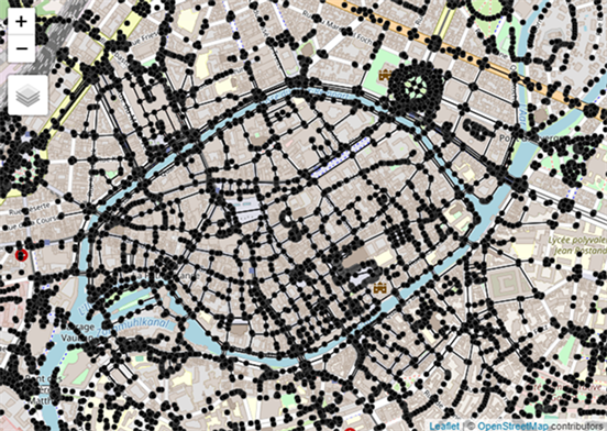
## Plot
tmap_leaflet(tm_shape(filtered %>% activate(edges) %>% as_tibble() %>% st_as_sf()) +
tm_lines() +
tm_shape(filtered %>% activate(nodes) %>% as_tibble() %>% st_as_sf()) +
tm_dots() +
tmap_options(basemaps = 'OpenStreetMap'))
Step 3- Load the spatial location of origins/destinations (frequented location)
The following code is used for importing the input data file: spatial location of origins/destinations. These data need to import in separate table one for origin addresses and another one for destination addresses. Each table as data.frame should contain the columns id, long and lat.
## Starting addresses
geo1 <- tibble(token = c(1,2),
lon = c(7.64895,7.73657),
lat = c(48.58591,48.63136)
)
## Arrival addresses
geo2 <- tibble(token = c(1,2),
lon = c(7.74636,7.76416),
lat = c(48.58842,48.53916)
)
geo1 <- data.frame(token= geo1$token,"lon_from"=geo1$lon, "lat_from"= geo1$lat) %>%
st_as_sf(coords = c("lon_from", "lat_from")) %>%
st_set_crs(st_crs("WGS84"))
geo2 <- data.frame(token= geo2$token,"lon_from"=geo2$lon, "lat_from"= geo2$lat) %>%
st_as_sf(coords = c("lon_from", "lat_from")) %>%
st_set_crs(st_crs("WGS84"))
## Plot
tmap_leaflet(tm_shape(geo1 %>% as_tibble() %>% st_as_sf()) +
tm_dots() +
tm_shape(geo2 %>% as_tibble() %>% st_as_sf()) +
tm_dots(col="red") +
tm_add_legend(labels = c("Starting addresses","Arrival addresses "),col = c("black","red")) +
tmap_options(basemaps = 'OpenStreetMap'))

Step 4- Build a final road network containing origin and destination point
The following code is used to merge the addresses to the road network and to obtain a more precise calculation of the route.
graph <- graph %>% # activation of the network nodes
activate(nodes)
r <- as_tibble(graph) #we change the format
l<- length(r$nodesID) + 1#we evaluate the number of existing nodes
rm(r) #we delete the object R, we don’t need it anymore
geo1 <- geo1 %>% # we give an identifier to the starting addresses which takes into account the nodes already existing in the network
mutate(from=seq(l,l+1)) # there were already 249 020 nodes so the two new ones will be 249 021 and 249 022
geo2 <- geo2 %>% # same with the arrival addresses which come after the departure addresses so 249 023 and 249 024
mutate(to=seq(l+2,l+2+1))
g1= geo1 %>% #we create a sub-file containing only the geographical coordinates and the newly created identifiers
rename(nodesID=from) %>%
select(-token)
graph <- graph %>%
activate(edges)
blended = st_network_blend(graph, g1) #fusion
## technical and aesthetic treatments
blended = blended %>%
activate(nodes)
blended <- mutate_at(blended, c("nodesID.x","nodesID.y"), ~replace(., is.na(.), 0))
blended = blended %>%
mutate(nodesID= ifelse(`nodesID.x`==0, as.numeric(`nodesID.x`) + as.numeric(`nodesID.y`),
ifelse(`nodesID.x`!=0,`nodesID.x`,
NA))) %>%
select(-`nodesID.x`)
t<- as_tibble(blended)
t <- t %>%
filter(`nodesID.y`!=0)
t1 <- t$nodesID.y
t2 <- t$nodesID
t <- cbind(t1,t2)
t <- as_tibble(t)
t <- t[order(t1),]
t <- t %>%
rename(nodesID=t1) %>%
rename(from=t2)
geo1 <- geo1 %>%
rename(nodesID=from)
##
geo1 <- merge(geo1,t,all.x=TRUE) #we get the identifier of the newly added nodes to be able to call them later,
# if an address had already been present, the old name would have been kept
graph = blended #the new graph contains the starting addresses
## We proceed in the same way with the arrival addresses on the newly created graph
graph <- graph %>%
select(-nodesID.y)
g2= geo2 %>%
rename(nodesID=to) %>%
select(-token)
graph <- graph %>%
activate(edges)
blended = st_network_blend(graph, g2)
blended = blended %>%
activate(nodes)
blended <- mutate_at(blended, c("nodesID.x","nodesID.y"), ~replace(., is.na(.), 0))
blended = blended %>%
mutate(nodesID= ifelse(`nodesID.x`==0, as.numeric(`nodesID.x`) + as.numeric(`nodesID.y`),
ifelse(`nodesID.x`!=0,`nodesID.x`,
NA))) %>%
select(-`nodesID.x`)
t<- as_tibble(blended)
t <- t %>%
filter(`nodesID.y`!=0)
t1 <- t$nodesID.y
t2 <- t$nodesID
t <- cbind(t1,t2)
t <- as_tibble(t)
t <- t[order(t1),]
t <- t %>%
rename(nodesID=t1) %>%
rename(to=t2)
geo2 <- geo2 %>%
rename(nodesID=to)
geo2 <- merge(geo2,t,all.x=TRUE)
graph = blended
At the end of this step, the new road network contains the origin and destination point. The followings code allows us to create the final file which will be use to calculate the routes.
lieu1 <- tibble(token=c(1,1,2), # creation of a table with two individuals, 1 and 2
mode=c("walk","car","car"), # woman 1 uses the pedestrian and car mode, woman 2 only her car
temps2=c(333.3340,25000.0500,16666.7000)) # here transport times converted into distance, 5min walk...
token <- geo1$token
from <- geo1$from
from <- cbind(token,from)
from <- as_tibble(from)
token <- geo2$token
to <- geo2$to
to <- cbind(token,to)
to <- as_tibble(to)
lieu1$token <- as.numeric(lieu1$token)
lieu1 <- left_join(lieu1,from)
lieu1 <- left_join(lieu1,to)
un_fichier <- lieu1 %>%
filter(!is.na(from)) %>%
filter(!is.na(to))
head(un_fichier)
Step 5- Creation of several “node libraries”
In order to create several “node libraries”, the user need to load a set of function:
source("~/Documents/…/algo2.R")
source("~/Documents/…/gros_algo.R")
source("~/Documents/…/res_bus.R")
source("~/Documents/…/res_tram.R")
source("~/Documents/…/f_gen.R")
The following code is used to create several “node libraries” needed for multimodal trip (also use in unimodal trip).
edges <- graph %>%
activate(edges) %>%
as_tibble()
walk <- as_tibble(edges$walk)
car <- as_tibble(edges$car)
bicycle <- as_tibble(edges$bicycle)
from <- as_tibble(edges$from)
to <- as_tibble(edges$to)
walk <- rename(walk, walk = value)
car <- rename(car, car = value)
bicycle <- rename(bicycle, bicycle = value)
from <- rename(from, nodesID = value)
to <- rename(to, nodesID = value)
temp1<-cbind(from,walk,car,bicycle)
temp2<-cbind(to,walk,car,bicycle)
nodes <- graph %>%
activate(nodes) %>%
as_tibble()
nodes_bus <- graph_transit_und %>%
activate(nodes) %>%
select(c(nodesID_bus,nodesID)) %>%
as_tibble()
nodes_bus <- nodes_bus[!(is.na(nodes_bus$nodesID_bus)),]
ligne <- graph_transit_und %>%
activate(edges) %>%
select(c(from,id_ligne)) %>%
rename(nodesID=from)%>%
as_tibble()
nodesID <- as_tibble(ligne$nodesID)
id_ligne <- as_tibble(ligne$id_ligne)
nodesID <- rename(nodesID, nodesID=value)
id_ligne <- rename(id_ligne, id_ligne=value)
ligne <- cbind(nodesID,id_ligne)
nodes_transit <- inner_join(nodes_bus,ligne, by="nodesID")
st_crs(nodes_bus)="WGS84"
temp1 <- temp1 %>%
distinct(nodesID, .keep_all = TRUE)
temp2 <- temp2 %>%
distinct(nodesID, .keep_all = TRUE)
test_dep <-left_join(nodes,temp1, by="nodesID")
test_ar <- left_join(nodes,temp2,by="nodesID")
Step 6- Creation of set of routes
The following code is used to create a set of routes
nodes <- graph %>%
activate(nodes) %>%
as_tibble()
fin <- fonction_gen(un_fichier)
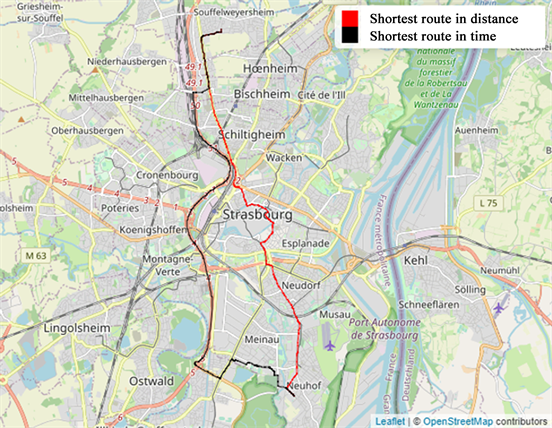
Visualize results
The user can visualize multiple alternative routes between origin/destination pairs in geographic context using following code. In our example (pregnant women ID 2), we visualize the shortest route with heavy traffic.
tmap_leaflet(
tm_shape(fin[fin$id==2& fin$met=="length",] %>% as_tibble() %>% st_as_sf()) +
tm_lines(col="red") +
tm_shape(fin[fin$id==2& fin$met=="time",] %>% as_tibble() %>% st_as_sf()) +
tm_lines() +
tm_add_legend(labels = c("Shortest route in distance","Shortest route in time"),col =c("red","black")) +
tmap_options(basemaps = 'OpenStreetMap'))
Step 7- Calculation of daily concentration
To calculate daily concentrations, the user needs to load the R objects
In this example, we calculate the average concentrations for several fictive itineraries traveled by several fictive pregnant women “id” using the followed code:
load("grille.RData") # loading the grid: 2 columns, the geometry in polygons and an identifier
# here it is not unique because several grid squares will share the same pollution values due to a limited number of monitoring stations
load("letsgo.RData") # the letsgo file is from the previous algorithm
load("releve.RData")# a survey file that at least contains a concentration at a given time, day, and grid tile
load("temp.RData") # "temp" contains trip information with, at least, an ID associated with a departure time
letsgo <- letsgo[c(1,2,3,4,5,7,8,9,10,11,12),]
library(dplyr)
library(sfnetworks)
library(lwgeom)
library(mapview)
temp$id <- as.character(temp$id)
simple <- left_join(letsgo,temp) # add the info from "temp" to "letsgo
travail <- as_tibble(simple)
travail <- travail[,-8]
travail$c <- 0# create a column that will receive the value of the concentration
releve <- as_tibble(releve)
releve$pol <- as.numeric(releve$pol)
pollution <- function(simple,travail,grille){
g=grille
r <- length(simple$id)
for (i in1:r){
t<-st_split(simple[i,],grille) # cutting of the itinerary according to the grid
h<-st_collection_extract(t,"LINESTRING")
h <- as_tibble(h)
h <- h %>%
st_as_sf
st_crs(h) <- "WGS84"
# Each new segment is attached to the nearest grid tile, which is the one in which the segment is located
h <- h %>% dplyr::mutate(id=st_nearest_feature(h,g))
h <- h %>%
dplyr::mutate(id_pol = g[id,]$id)
h <- h %>%
mutate(length = st_length(x))
# recovery of the departure time and the day
heure_dep <- h[1,]$h1
jour_dep <- h[1,]$jour
releve2 <- releve %>%
filter(jour==jour_dep)%>%
filter(heure==heure_dep)
# average of the concentrations per grid tile because several values/stations are sometimes present in a tile
releve2 <- releve2 %>%
group_by(id)%>%
summarise(mean(pol))
releve2 <- releve2 %>%
rename(id_pol=id)
h <-left_join(h,releve2)
h <- h %>%
rename(concentration=`mean(pol)`)
# new variable that is the product of each segment in h and the associated tile concentration to the segment
h <- h %>%
mutate(c=length*concentration)
tadam <- sum(h$c)/sum(h$length)
p <- simple[i,]$id
q <- simple[i,]$met
travail[travail$met==q & travail$id==p & travail$jour==jour_dep & travail$h1==heure_dep,]$c <- as.numeric(tadam)
}
return(travail)
}
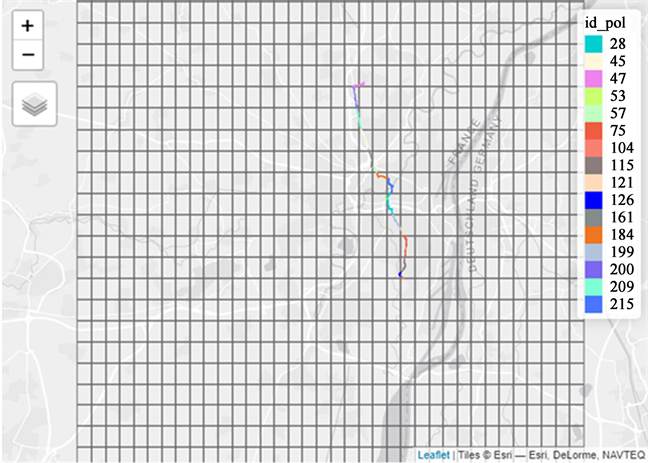
At the end of this step, each segment of the route is associated with a cell of the grid.
The following code will allow attributing, for a given hour and a given day, either the concentration of pollutant modeled at the cell of grid-scale or the concentration of pollutant measured by the nearest monitoring station (Table 1).
result <- pollution(simple,travail,grille)
![]()
Table 1. Extract from the result table.
Extract from the result table met: method of itinerary calculation, temps: transport duration, mode: mode of transport, id: identifier, h1 and h2: hour of arrival and departure, c = Individual daily exposure assessment.
6. Conclusions
In this paper, we have presented the tool designed to ease the calculation of the daily air pollutants exposure taking into account the individual spatiotemporal activity. To our knowledge, no such reproducible procedure had previously been proposed.
This paper makes an important contribution by presenting a new procedure that supplies researchers with a useful tool to calculate daily exposition to air pollutants. The procedure integrates the time spent at frequented locations (work, shopping, residential address, etc.) and while commuting, which require the efficient calculation of travel time matrices or the examination of multimodal transport routes with open-source code.
One strength of the tool is that the procedure can be used with different spatial scales and for any air pollutant. For instance, if input data of air pollution are modeled at square grid or census block level, or measured in the monitoring station, daily exposure can be readily estimated.
As a domain of application for future work, the procedure could be used to extend the estimation of air pollution to any participant (not only pregnant women). We believe that this tool will be used in various areas. This could improve the estimation of health effects related to air pollution exposure and will also allow the identification of windows of vulnerability. Moreover, this work will continue to be exploited and developed in the framework of future research. The next step is to create an R package to simplify the application of the procedure for non-specialists.
Acknowledgments
This paper was supported Ph.D. student grant by the Region Grand Est.
This work is supported by IRESP. (Public Health Research Institute GIS-IRESP)
The funder had no role in study design, data collection, analysis, decision to publish, or preparation of the manuscript.