Maximum Power Point Tracking Using the Incremental Conductance Algorithm for PV Systems Operating in Rapidly Changing Environmental Conditions

Derek Ajesam Asoh^1,2,3*, Brice Damien Noumsi⁴, Edwin Nyuysever Mbinkar¹

¹Laboratoire de Génie Electrique, Mécatronique et Traitement du Signal, ENSPY, University of Yaounde I, Yaounde, Cameroon.
²Department of Electrical/Electronic Engineering, NAHPI, University of Bamenda, Bamenda, Cameroon.
³Higher Technical Teacher Training College (HTTTC), University of Bamenda, Bamenda, Cameroon.
⁴Department of Electrical/Electronics Engineering, Nigeria Army College of Environmental Studies and Technology (NACEST), Makurdi, Nigeria.

DOI: 10.4236/sgre.2022.135006                

Abstract

Maximum Power Point Tracking (MPPT) is an important process in Photovoltaic (PV) systems because of the need to extract maximum power from PV panels used in these systems. Without the ability to track and have PV panels operate at its maximum power point (MPP) entails power losses; resulting in high cost since more panels will be required to provide specified energy needs. To achieve high efficiency and low cost, MPPT has therefore become an imperative in PV systems. In this study, an MPP tracker is modeled using the IC algorithm and its behavior under rapidly changing environmental conditions of temperature and irradiation levels is investigated. This algorithm, based on knowledge of the variation of the conductance of PV cells and the operating point with respect to the voltage and current of the panel calculates the slope of the power characteristics to determine the MPP as the peak of the curve. A simple circuit model of the DC-DC boost converter connected to a PV panel is used in the simulation; and the output of the boost converter is fed through a 3-phase inverter to an electricity grid. The model was simulated and tested using MATLAB/Simulink. Simulation results show the effectiveness of the IC algorithm for tracking the MPP in PV systems operating under rapidly changing temperatures and irradiations with a settling time of 2 seconds.

Keywords

Modeling, Simulation, PV System, Maximum Power Point Tracking (MPPT), Incremental Conductance Algorithm, MATLAB/Simulink

1. Introduction

As we head into the end of the first quarter of the 21^st century, harnessing and exploitation of various renewable energy sources and systems, has emerged as an imperative for all round sustainable development and growth of nations [1]. Among the various sources of renewable energy (hydro, wind, solar, biogas etc.), solar is the only source that is available everywhere and is free to harness and exploit [2]. Solar energy can be harnessed through two technologies: photovoltaic (PV) and thermal. PV technology uses solar cells which exhibit photovoltaic (PV) effect to convert sunlight into electricity in what is referred to as solar PV systems; while thermal technology converts the energy in sunlight into heat that can be used in various heat demanding applications, in what is referred to as solar thermal systems.

The use of solar PV systems as a source for generating electricity has gained more ground than any other renewal renewable energy source in recent years. This is not only because the energy from the sun is free and omnipresent but also because of the sharp drop in the acquisition costs of PV System components and the simple energy solutions they provide [3]. Furthermore, low operation and maintenance costs, and the environmental friendliness of the technology by virtue of pollution-free operations have significantly propelled the popularity of solar PV systems [4] [5], which have evolved significantly from small standalone to large grid connected systems [6].

Solar PV systems in use are exploited either in standalone or in grid connected configurations [3] [7]; and have wide applications for electricity supply in remote villages and rural communities of developing country environments [3]. Irrespective of the configuration of the PV system the I-V curve upon which the power output of the system depends is non-linear [8]. Furthermore, the P-V curve of PV systems is also non-linear and in cases of mismatched conditions, for example, different orientations of PV panels belonging to the same PV field, manufacturing tolerances, and non-uniformity of ambient temperatures, the P-V curve may have more than one peak [4]. The implication of this non-linearity is that there is a unique point on the curve, called the Maximum Power Point (MPP) which needs to be tracked to ensure that the system operates at maximum efficiency and produces maximum power output [5]. Besides the non-linearity of the I-V curve, PV systems in general have low efficiencies in practice [6] [7]; and the MPP varies with changes in solar insolation and other environmental factors, including partial shading of the solar cells [7]; and hence a need for tracking to ensure maximum power output [5].

For solar PV systems to remain a competitive energy source among the renewables, it is necessary to extract the maximum power from each panel and lower the cost per kilowatt [2]. Extracting the maximum possible power from a PV system cannot result from a simple interconnection of components. Many environmental variables affect the performance of a PV panel, including dust, shades, shadows, irradiation levels, and ambient temperature [2] [9]. Without the ability to track and extract maximum power from a PV system, the system may not be sustainable [8].

This study focuses on modeling, simulating, and testing the Incremental Conductance (IC) Algorithm for maximum power point tracking (MPPT) in PV systems operating under rapidly changing environmental conditions. By modeling and simulating, the expectation is to ensure that the MPPT algorithm being implemented can deliver to the level of ensuring a sustainable PV system. The rest of this paper is organized as follows. Section 2 is a brief overview of MPPT techniques and algorithms relevant to the study. Section 3 focuses on the methods and materials of the study. Simulation results are presented in Section 4 and analyzed to validate the effectiveness of the Incremental Conductance (IC) Algorithm for maximum power point tracking (MPPT) and control of PV systems operating under rapidly changing environmental conditions such as temperature and irradiation. This is followed by concluding remarks and direction for future research in Section 5.

2. Maximum Power Point Tracking (MPTT) Algorithms

With the desire for more efficient and low-cost PV systems, many maximum power point tracking (MPPT) techniques/algorithms/methods have been developed since the last decades. Some of the techniques/algorithms/methods have been optimized for even greater power output. Comparative studies of the MPPT techniques/algorithms/methods have been widely analyzed and compared [4] [5] [10] [11] [12] [13] [14]. We present an overview to enable us make a choice for this study.

In an extensive study, Subudhi and Pradhan [4] identified and classified 26 different MPPT techniques/algorithms/methods. Their classification was based on a number of features, including number of control variables involved, types of control strategies, circuitry, cost, parameter tuning, complexity level, converter used (DC, AC, or both), and application configuration area (standalone and grid connected). While these authors make important pronouncements on the suitability or non-suitability of some of the techniques/algorithms/methods, it is important to note that the criteria used in the classification is generic and has a much wider application. The criteria can be helpful in selecting current and future MPPT techniques/algorithms/methods for particular applications. For example, it is cheaper to implement an MPPT technique/algorithm/method based on voltage as a single control variable compared to using current as the control variable.

Babaa et al. [5] identified and investigated various types of MPPT techniques/algorithms/methods, including perturbation and observation (P&O), incremental conductance (IC), constant voltage (CV), temperature (T), open voltage (OV), feedback voltage (current), fuzzy logic control (FLC), and neural network (NN). The performance of each MPPT technique/algorithm/method was evaluated in terms of ease of implementation, cost of implementation, ability to detect multiple maxima, speed of convergence, and efficiency over a wide range of power outputs. These authors found that the incremental conductance (IC) and the perturbation and observation (P&O) techniques ensured that the MPP is not only quickly tracked but also very importantly, they minimize ripples around the MPP thereby ensuring maximum power output. Furthermore, these two techniques were noted to be the most suitable for use in PV systems because they are easy to implement and are more effective when the PV system implementation objective is to reduce payback period. In fact Dolara et al. found that the P&O and IC methods have the same cost and software overheads [15].

The aforementioned findings, which agree with work reported by Subudhi and Pradhan [4], give credit to the P&O and IC as the preferred and most viable algorithms for implementation of MPPT in PV systems. The P&O and IC methods have recently been identified as direct tracking methods whose operations point is independent of isolation, temperature, or degradation levels because they can be effected without prior knowledge of the I-V characteristics of the PV system [7].

Despite the high standing of the P&O and IC algorithms compared to other techniques/algorithms/methods, the IC algorithm is considered a better alternative to the P&O in applications characterized by dynamic environmental conditions such as high, fast and continuously changing light levels during which the P&O algorithm is more prone to errors [15]. Based on the fore going discussions and its advantages, the IC algorithm is selected for this study.

3. Methods and Materials

The problem addressed by using MPPT algorithms is how to automatically find the respective voltage (Vmpp) and/or current (Impp) at the Maximum Power Point (MPP), where a PV system should operate in order to produce maximum electrical power output within specific environmental conditions (irradiance, temperature, etc). In this study, modeling and simulation of the selected algorithm was done in MATLAB/Simulink. The implementation was effected by inserting a DC-DC converter between the PV panel and the load as recommended by Baimel et al. [7] and York et al. [16]. In effect, a controller was embedded in the power electronic converter systems in such a way that the corresponding optimal duty cycle is updated to the photovoltaic power conversion system to generate the maximum power output. Details are presented in the following subsections

3.1. Block Diagram of the Proposed System

The physical components of the system for the implementation of the incremental conductance (IC) MPPT algorithm is shown in Figure 1 [2].

The system consists of a solar PV panel, DC-DC boost converter, MPPT control loop and duty cycle adjustment, voltage sensor, current sensor, PWM generator, 3-phase VSC, 3-phase VSC controller, and the utility grid/load. The switching of DC-DC boost converter is controlled by IC MPPT algorithms using a Pulse Width Modulation (PWM) generator [7]. The output current and voltage of the solar panel are sensed and fed to the MPPT controller. The MPPT controller modulates the duty cycle of the PWM to maintain a steady output current and voltage of the DC-DC boost converter. The adjustment of the duty cycle fed to the boost converter provides maximum power. The boost converter works based on these pulses to make the PV system operate at maximum power point (MPP). The Voltage Source Converter (VSC) converts the output voltage of the boost converter and supplies it to the grid.

3.2. The Solar Cell

Solar cells are the building blocks of PV panels or modules, which in turn are building blocks for the PV arrays used in PV systems. In operation, a solar cell is considered as a two terminal device with characteristic behavior as a diode (single diode model) and the ability to convert energy of sunlight photons to electrical energy. The equivalent circuit of the general model then consists of a photocurrent, a diode, a parallel resistor expressing a leakage current, and a series resistor describing an internal resistance to the current flow is shown in Figure 2, and I-V characteristic depicted by Equation (1) [2] [6] [17].

$I=I_{ph}-I_0\left[\exp \left\{\frac{q\left(v+R_{s}I\right)}{nKT}\right\}-1\right]-\left[\frac{V+R_{s}I}{R_{sh}}\right]$ (1)

Figure 1. Block diagram of the proposed system [2].

Figure 2. Equivalent circuit of PV solar cell [2] [6] [17].

where,

I_ph is the photocurrent (in amperes);

I₀ is the reverse saturation current (in amperes);

R_s is the series resistance (in ohms);

R_sh is the parallel resistance (in ohms);

N is the diode factor;

q is the electron charge = 1.6 × 10⁻¹⁹ (in coulombs);

K is Boltzmann’s constant (in Joules/ Kelvin);

T is the panel temperature (in Kelvin);

V is the cell output voltage (in Volts).

Given that the power generated by a solar cell based on the I-V curve of Equation 1 is quite small (about 45 mW), these cells are connected in series or in parallel to obtain substantial electrical power for the PV panel required application [9]. As can be observed from Equation (1), the I-V curve for a PV cell is non-linear and is influenced by solar irradiance level, ambient temperature, wind speed, humidity, pressure, etc. The irradiation and ambient temperature are the two primary factors considered in this study.

As prelude to model and simulate the IC algorithm, the output characteristics of PV cell was first obtained in simulation experiments. For constant temperature (25˚C) and different irradiation intensities (400 - 1000 W/m²), the PV cell current was maintained constant while the voltage varied up to some voltage level and then subsequently decreased. Table 1 shows the solar panel specifications used in this work.

3.3. The Boost Converter

The boost converter was modeled before the simulation in MATLAB. The boost converter was designed with due consideration for low cost, simplicity, and efficiency. The equivalent circuit of the boost converter is presented in Figure 3 [2], with V_d and V_o as input and output voltages respectively. Numerical values of components such as inductor, capacitor, and resister were determined from circuit analysis with the circuit premised on a continuous conduction mode.

The boost converter operates in two modes: charging and discharging modes. These two modes of operations are based on the ON and OFF position of the switch, S. The charging mode occurs when the switch is closed (ON); while the discharging mode occurs when the switch is opened (OFF).

During the charging mode, the switch is closed and the inductor is charged by the source through the switch. At this time, the diode is reverse-biased and as such separates the converter into two sections. The rate of change of inductor current is constant, demonstrating a linearly increasing pattern of inductor current. The equivalent circuit of the boost convertor in the charging mode is depicted in Figure 4.

When S is closed (ON) as shown in Figure 4, the following equations are applicable to the boost converter circuit: The input voltage of the boost converter is considered as V_d

Figure 3. The ideal boost converter [2].

Table 1. PV Panel characteristics and specifications (Model SunPower SPR-305E-WHT-D).

Figure 4. Equivalent circuit of boost converter with switch closed [2].

$V_d=V_l$ (3)

$V_d=L\frac{di}{dt}$ (4)

$V_d=L\frac{I_{\max }-I_{\min }}{dt}$ (5)

$\frac{V_d}{L}dt=I_{\max }-I_{\min }$ (6)

$I_{\max }=I_{\min }+\frac{V_d}{L}dt$ (7)

The equivalent circuit of the boost convertor in the discharging mode is shown in Figure 5.

When S is open (OFF) as shown in Figure 5, the following equations are applicable to the boost converter circuit:

$-V_d+V_L+V_0=0$ (8)

$V_0=V_d-V_L$ (9)

But $V_L=L\frac{d{i}_L}{dt}$ (10)

$V_0=V_d-L\frac{d{i}_L}{dt}$ (11)

$V_0=V_d-L\frac{I_{\min }-I_{\max }}{T-dT}$ (12)

$-L\frac{I_{\min }-I_{\max }}{\left(I-d\right)T}=V_0-V_d$ (13)

$I_{\min }-I_{\max }=\frac{V_d-V_0}{L}\left(I-d\right)T$ (14)

$I_{\max }=I_{\min }-\frac{V_d-V_0}{L}\left(I-d\right)T$ (15)

$I_{\max }=I_{\min }+\frac{V_0-V_d}{L}\left(I-d\right)T$ (Since $V_0>V_d$ ) (16)

Making (7) = (16) (17)

$I_{\min }+\frac{V_d}{L}dT=I_{\min }+\frac{V_0-V_d}{L}\left(I-d\right)T$ (18)

$V_{d}dT=\left(V_0-V_d\right)\left(I-d\right)T$ (19)

Figure 5. Equivalent circuit of the boost converter when switch opened [2].

$\frac{V_0}{V_d}=\frac{I}{I-d}$ (20)

From the models and equations of the boost converter presented above, we simulated the boost converter in MATLAB/Simulink as presented in Figure 6.

3.4. The Incremental Conductance (IC) Algorithm

With the IC algorithm, the PV panel terminal voltage is adjusted according to the MPP voltage. When the IC algorithm determines that the MPP has been reached, it settles and stops moving around the operating point. The MPP is achieved by comparing the instantaneous conduction (I/V) to the incremental conductance (∆I/∆V). Being able to determine when the MPP has been reached is possible because the relationship dP/dV is negative when the MPPT is to the right of the MPP and positive when it is to the left of the MPP. In effect, the IC algorithm examines the slope of the PV array power characteristics to track MPP; and when the slope of the PV panel power curve is zero, the MPP is established.

For the IC flow chart shown in Figure 7, the following equations are applicable:

$dP/dV=0$ for $V=V_{mp}$ , (21)

$dP/dV>0$ for $V<V_{mp}$ , (22)

$dP/dV<0$ for $V>V_{mp}$ . (23)

The fact that P = IV and the chain rule for the derivative of products yields:

$dP/dV=d\left(VI\right)/dV=IdV/dV+VdI/dV=I+VdI/dV$ (24)

Combining Equations (21) and (22) leads to the MPP condition ( $V=V_{mp}$ ) in terms of array voltage V and array current I:

$dI/dV=-I/V$ . (25)

3.5. Voltage Source Converter (VSC)

A three-level Voltage Source Converter (VSC) regulates the DC bus voltage at

Figure 6. The boost converter in MATLAB.

Figure 7. Flowchart of Incremental Conductance (IC) algorithm.

500 V and keeps unity power factor. The control system uses two control loops: an external control loop which regulates DC link voltage to ±250 V and an internal control loop which regulates Id and Iq grid currents (active and reactive current components). The Id current reference is the output of the DC voltage external controller. The Iq current reference is set to zero in order to maintain unity power factor. The Vd and Vq voltage outputs of the current controller are converted to three modulating signals Vref-abc, which are used by the PWM three-level pulse generator. The control system uses a sample time of 100 µs for the voltage and current controllers as well as for the PLL synchronization unit. In a more demanding application model, the pulse generator for the boost and VSC converter uses a faster sample time of 1 μs in order to get an appropriate resolution of PWM waveforms.

Internal to the VSC, a universal bridge block implements a universal three-phase power converter which consists of six power switches (S1, S2, … S6) connected in a bridge configuration (see Table 2, next subsection). The type of power switch and converter configuration is selectable from the simulation dialog box. The universal bridge block allows simulation of converters using either naturally commutated (or line-commutated) power electronic devices (diodes or thyristors) and forced-commutated devices (MOSFET).

For this study, the boost and VSC converters models are represented by equivalent voltage sources generating the AC voltage averaged over one cycle of the switching frequency. Such a model does not exhibit harmonics, but the dynamics resulting from the interaction of the control and power systems are preserved.

Table 2. 3-Level inverter switching table.

These models make it possible to use larger time steps than in more demanding application model (i.e. 50 µs vs. 1 µs), resulting in a much faster simulation [18].

3.6. Switching Table

The switching table is formed using the sector, corresponding voltage vector, and switch state. For example, if the angle of the reference voltage is between 0˚ and 60˚, it is in sector 1 and it selects the voltage vector V1. The summary of various switching states (S1, S2, …, S6) and associated voltages is given in Table 2.

4. Simulation Results and Discussions

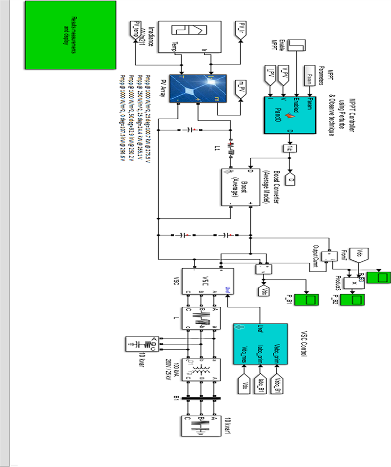
Simulations were conducted using MATLAB/Simulink in order to test the functionality and performances of the IC algorithm. The complete circuit diagram of the MPPT circuit and the simulation results is shown in Appendix 1. The performance outputs of the various segments of the design circuits were simulated and analyzed after selection of components, both active and passive

4.1. Simulation of Temperature and Irradiations

Figure 8 shows the irradiance and temperature variations generated as inputs for the PV panel operation. In this figure, the irradiance is generated at a constant value of 1000 Kw/m² for 0.5 s second, then decreased at 250 Kw/m² for 0.5 s and maintained constant for another 0.5 s. Subsequently the irradiation increases steadily from 250 Kw/m² to 1000 Kw/m² after 2 s and is maintained constant for the rest of the simulation.

Next we simulated the behavioral pattern of temperature variation on the PV panel. Maintained at an initial constant temperature of 25˚C (room temperature) for a period of 2 s, the temperature was steadily increased to an extreme value of 50˚C after 3 s and maintained at this value for 1 s. Subsequently, the temperature was steadily decreased to 0˚C after another 1 s. The foregoing steps

Figure 8. Irradiance and temperature variations.

Figure 9. I-V curve (at 25˚C and 1000, 800, 600 and 400 W/m² respectively).

were repeated for various combinations of irradiation and temperature variations., typical conditions in a changing environment. The presentation and discussions of the resultant I-V and P-V curves follows

4.2. I-V Curves and P-V Curves for the PV Panel

Figure 9 depicts the I-V curve for the PV panel model Sunpower SPR 305-WHT-D 100 kW and IMMP of 5.58 A at 1000 kW/m² irradiance. It can be seen that the photo-generated current is directly proportional to the irradiance as the voltage increases. The graph shows changes in the value of irradiance from 1000 kW/m², 800 kW/m², 600 kW/m² to 400 kW/m² respectively with the temperature fixed at 25˚C.

With a fixed temperature of 25˚C and variation of irradiance as 1000 kW/m², 800 kW/m², 600 kW/m², and 400 kW/m², we obtained the P-V curve of Figure 10. From this figure, we note that the power output of the PV panel is directly related to the irradiance; the voltage output increases as the irradiance increases until a threshold value is attained, at the Maximum Power Point (MPP) after which it decreases.

Figure 11 shows the output signal of the I-V curve with fixed irradiance (1000 kW/m²) at 0˚C, 25˚C, 30˚C, 35˚C, 40˚C, 45˚C respectively. Observations from the curve shows that increment in the ambient temperature slightly affect the voltage level of the PV system.

Similarly, in Figure 12, a plot of the P-V curve with fixed irradiance (1000

Figure 10. P-V curve (at 25˚C and 1000, 800, 600 and 400 W/m² respectively).

Figure 11. I-V curve at 1000 W/m² with different temperatures.

kW/m²) at 0˚C, 25˚C, 30˚C, 35˚C, 40˚C, 45˚C respectively shows how variations in temperature can affect the power output of the PV panel. As the temperature gradually decreases, the power generated at the output of the modules also increases thereby causing a change in the MPP of the system.

Table 3 shows the values of current, voltage, and power obtained when the irradiance is varied from 1000 kW/m², 800 kW/m², 600 kW/m² to 400 kW/m² with a fixed temperature of 25˚C (room temperature), while Table 4 shows the same values when the irradiance is constant at 1000 kW/m².

Figure 12. P-V curve at 1000 W/m² with different temperatures.

Table 3. MPP at 25˚C with different irradiation levels.

Table 4. MPP at 1000 kW/m² with different temperatures.

4.3. Results Using the Incremental Conductance (IC) Algorithm

Figure 13 shows the current, voltage and power output of the DC converter over 2.5 s.

Figure 13 shows the current, voltage and power output respectively with IC algorithm. Variations are observed at at different intervals which can be attributed to the variations in irradiance. The settling time $t_s$ for the technique is $t_s=0.2\text{s}$ . At the beginning of the simulation, it can also be seen that there is a delay caused by transients. The results also show that the sudden change in irradiation also affects the power output of the boost converter. Figure 14 shows the duty cycle as it varies with the change in irradiance and temperature, but is still maintained within the range of 0 to 1 s, which shows that the MPP is tracked at all points.

4.4. Results from the Voltage Source Converter with the IC Algorithm

Figure 15 shows the phase voltage and current respectively, while Figure 16 shows the power at the Voltage Source Converter output of a system using IC algorithm. The results in these figures show similar output in terms of amplitude

Figure 13. Current, voltage and power output (from top downward) with IC MPPT technique.

Figure 14. Duty cycle with IC algorithm.

Figure 15. Current, voltage, and output respectively with IC algorithm.

for both voltage and current. The variations in power output are due to the changes in irradiance.

5. Conclusions

Many techniques/algorithms/methods have been proposed and used in the

Figure 16. Output power with IC algorithm.

tracking MPP for the efficient operation of PV systems. Selecting a particular MPPT technique/algorithm/method for a system calls for diligent consideration of cost, reliability, speed, accuracy, and efficiency of the system. The power ratings of PV panel and climate conditions are also factors in certain areas and in some applications.

From an overview of the literature, this study identified the P&O and IC algorithms as the most robust ones to use for tracking of MPP in PV systems. The IC algorithm was preferred and selected for the study because it outperforms the P&O algorithm when the requirement is operation in fast changing dynamic environmental conditions such as temperature and irradiance levels.

Starting with the block diagram, all components of the system required for the modeling and simulation of the IC algorithm were elaborated and modeled, alongside with description of operation. Subsequently the system was simulated using MATLAB/Simulink. Simulation results were presented and discussed. Review and analysis of the results revealed the implementation of IC algorithm being effective for MPP tracking and control of the PV panel used in the study with a settling time of 2 s; and operating under varying environmental conditions of temperature and irradiation. These results cannot be generalized given that only one model of PV panel was used.

Direction of further studies includes replication of the study with different models of PV panels as well as using soft computing techniques.

Acknowledgements and Statement on Funding

The authors acknowledge and thank the authorities of the University of Yaounde I, the University of Bamenda, and the Nigeria Army College of Environmental Studies and Technology, Benue State, for their institutional support. The work was carried out as routine research and as such authors did not receive any funding for the work.

Appendix 1: Diagram of the Simulation of IC MPPT Algorithm for PV System

Conflicts of Interest

The authors declare no conflicts of interest regarding the publication of this paper.

References

[1]	Asoh, D.A., Mbinkar, E.N. and Moutlen, A.N. (2022) Load Frequency Control of Small Hydropower Plants Using One-Input Fuzzy PI Controller with Linear and Non-Linear Plant Model. Smart Grid and Renewable Energy, 13, 1-16. https://doi.org/10.4236/sgre.2022.131001
[2]	Noumsi, D.B., Ifeanyi, B.E. and Oladjo, M.C. (2019) Simulation of A Modified Perturb and Observe Algorithm for A Photovoltaic System Connected To the Grid. International Journal of Scientific Research & Engineering Trends, 5, 1052-1059.
[3]	Mbinkar, E.N., Asoh, D.A., Tchuidjan, R. and Baldeh, A. (2021) Design of a Photovoltaic Mini-Grid System for Rural Electrification in Sub-Saharan Africa. Energy and Power Engineering, 13, 91-110. https://doi.org/10.4236/epe.2021.133007
[4]	Subudhi, B. and Pradhan, R. (2013) A Comparative Study on Maximum Power Point Tracking Techniques for Photovoltaic Power Systems. IEEE Transactions on Sustainable Energy, 4, 89-98. https://doi.org/10.1109/TSTE.2012.2202294
[5]	Babaa, S.E., Armstrong, M. and Pickert, V. (2014) Overview of Maximum Power Point Tracking Control Methods for PV Systems. Journal of Power and Energy Engineering, 2, 59-72. https://doi.org/10.4236/jpee.2014.28006
[6]	Chouder, A., Silvestre, S., Sadaoui, N. and Rahmani, L. (2012) Modeling and Simulation of a Grid Connected PV System Based on the Evaluation of Main PV Module Parameters. Simulation Modelling Practice and Theory, 20, 46-58. https://doi.org/10.1016/j.simpat.2011.08.011
[7]	Baimel, D., Tapuchi, S. and Baime, N. (2017) New Improved Maximum Power Point Tracking Algorithm for Partially Shaded PV Systems. Journal of Power and Energy Engineering, 5, 55-63. https://doi.org/10.4236/jpee.2017.59005
[8]	Baramadeh, M.Y., Abouelela, M.A.A. and Alghuwainem, S.M. (2021) Maximum Power Point Tracker Controller Using Fuzzy Logic Control with Battery Load for Photovoltaics Systems. Smart Grid and Renewable Energy, 12, 163-181. https://doi.org/10.4236/sgre.2021.1210010
[9]	Rahmani, R., Seyedmahmoudian, M., Mekhilef, S. and Yusof, R. (2013) Implementation of Fuzzy Logic Maximum Power Point Tracking Controller for Photovoltaic System. American Journal of Applied Sciences, 10, 209-218. https://doi.org/10.3844/ajassp.2013.209.218
[10]	Femia, N., Lisi, G., Petrone, G., Spagnuolo, G. and Vitelli, M. (2008) Distributed Maximum Power Point Tracking of Photovoltaic Arrays: Novel Approach and System Analysis. IEEE Transactions on Industrial Electronics, 55, 2610-2621. https://doi.org/10.1109/TIE.2008.924035
[11]	Esram, T. and Chapman, P. (2007) Comparison of Photovoltaic Array Maximum Power Point Tracking Techniques. IEEE Transactions on Energy Conversion, 22, 439-449. https://doi.org/10.1109/TEC.2006.874230
[12]	Faranda, R. and Leva, S. (2008) Energy Comparison of MPPT Techniques for PV Systems. WSEAS Transactions on Power Systems, 3, 447-455.
[13]	Sera, D., Kerekes, T., Teodorescu, R. and Blaabjerg, F. (2006) Improved MPPT Method for Rapidly Changing Environmental Conditions. 2006 IEEE International Symposium on Industrial Electronics, Montreal, 9-13 July 2006, 1420-1425. https://doi.org/10.1109/ISIE.2006.295680
[14]	Femia, N., Petrone, G., Spagnuolo, G. and Vitelli, M. (2005) Optimization of Perturb and Observe Maximum Power Point Tracking Method. IEEE Transactions on Power Electronics, 20, 963-973. https://doi.org/10.1109/TPEL.2005.850975
[15]	Dolara, A., Faranda, R. and Leva, S. (2009) Energy Comparison of Seven MPPT Techniques for PV Systems. Journal of Electromagnetic Analysis and Application, 1, 152-162. https://doi.org/10.4236/jemaa.2009.13024
[16]	York, B., Yu, W. and Lai, J.-S. (2013) An Integrated Boost Resonant Converter for Photovoltaic Applications. IEEE Transactions on Power Electronics, 28, 1999-1207. https://doi.org/10.1109/TPEL.2012.2207127
[17]	Visweswara, K. (2014) An Investigation of Incremental Conductance Based Maximum Power Point Tracking for Photovoltaic System. Energy Procedia, 54, 11-20. https://doi.org/10.1016/j.egypro.2014.07.245
[18]	Noumsi, D.B., Nentawe, Y.G. and Manji, Y.M. (2016) Implementation of Maximum Power Point Tracking with a Boost Converter and a Three Level 3-Phase Inverter Connected to the Grid. International Journal of Innovative Research and Advanced Studies, 3, 319-325.