1. Introduction
There has been a global growth in the market for global healthcare Personal Protective Equipment (PPE) on COVID-19. The growth can be estimated between 2019 and 2020, from $5.99 billion in 2019 to $7.83 billion in 2020 (The Business Research Company, 2020). The key players in the PPE market include Lakeland Industries, 3M, Co., Honeywell International, Inc., Ansell Limited, Inc, E. I. DuPont de Nemours, and MSA Safety Co., Inc. The significant demand for PPE spiked after the COVID-19 outbreak and governments made effort to contain it. There is a supply and demand gap because of the restrictive containment measures. The dynamic market auction under the protective equipment on COVID-19 has been affected by the aforementioned reasons. The type of auction is a determinant of the way the bids are submitted in the bidding process. The dynamic auction takes place over several rounds where the bidders have a chance to watch as the action price develops and the other bidders bid (Allevi et al., 2016). The prices of commodities are relevant to the first-price auctions, making the market more dynamic. This model combines the competition over a period similar to the pairwise meeting models with instant bidding competitions. This model inquires how certain properties determine the relative significance of the two aspects, the competition and the way of the non-market clearing price, resulting from the bargaining and matching models affected by the bidding competition introduction (Hendricks & Sorensen, 2018). If the buyer’s valuations have heterogeneity to the commodities (PPE), then the discount factor is nearly 1 if the market remains frictionless. Without friction, there could be no competitiveness in the market and the non-market-clearing price result can be obtained. The agents present in the model are sellers and buyers of the PPE. The model shows how there is a mutual relationship between the buyer and the seller. The buyer is seeking commodity units owned by the seller. There is zero utility derived by the seller if they retain the good of the commodity unit forever. The buyer can assign significantly different values to different commodity units. The buyers are different also because their valuations for a given unit on sale are different (Liu & Sainathan, 2021). In pricing a given unit, in order to get a differentiable density, the consumption value that a given buyer assigns to a given unit is modeled as a random draw from a given distribution. The buyers match with the suitable sellers through distribution. Primarily, each buyer after realization of their valuation for a given PPE unit that they are facing and the number of buyers looking for a similar commodity in the bidding competition (Xue et al., 2018). After that, the buyer bids for the PPE unit. The seller determines the buyer whether the highest bidder or not; hence sell or retain a commodity (PPE) to have more value over time after receiving bids from different buyers. At the end of the given period, new buyers and sellers join the auction, and those who have completed transactions leave. This model for the dynamic market auction for the COVID-19 PPEs shows why it has been hard to determine the cost of the PPEs in a given region, because as timelines and periods change, the prices change since the people who are in higher demand will post a higher bidding price to win the bid (Lin et al., 2019). In fact, this later allows us to provide proof of known results for the extraction mechanism, and to extend these results to the “maximum match”, which constitutes a complete solution for the relevant auction system.
2. The Auction Mechanism
There is a set of bidders
and a set of items
, in the market in our auction mechanism, as well as a reservation price and v, which is the private value bidders. So price p is feasible if we suppose that there is a dummy item. The demand set by bidders at price p is:
the demand of bidder b at price p is competitive price if an allocation π is feasible and the pair
is an equilibrium when these conditions are satisfied: 1) each bidder is assigned only one item and every item to a one bidder; 2) if
and
then
; 3) similar items are sold same price; 4) if bidder b did not demand item j it means its upper price is equal to its selling price. If
, then
. π is an optimal matching if:
which maximizes welfare, so
is an efficient allocation of the items.Shapley and Shubik (Shapley & Shubik, 1971) demonstrated that a matching is an optimal if and only if it is competitive. The competitive equilibrium
is a maximum competitive equilibrium if
.
Definition 3.1: Auction Results Represented by a tuple of
, where
specifies the allocation number of items (
is the set of items assigned to player i) and
specifies Buyer’s payment (pi is the payment made by player i for distribution π).
Definition 3.2: Let p be the feasible price vector. Suppose that
, so
. set
and
then S is over-demanded at price
if
and
. the pair
is an equilibrium if:
• if
, then
;
• if
and
such that
then
;
• if
, then
.
In order to assign items to the bidders, in Step 1 the auctioneer announces the price of the items (reservation price), each bidder bids the item they want. if the price is not satisfied by the bidder then he/she chose dummy item which it has no value at all. Step2: the auctioneer finds the most needed item from the bidders as a minimum over demanded item and increases the price of that item with out changing the price of the other items. Step 3: if the price of the item is reached it’s upper bound price and there is only one bidder demanded that item then assign the item to that bidder but if
then decrease the price and allocate to the bidder. if there is an over demand then proceed Step 2.
3. Design and Analyze Algorithm of Maximum Matching
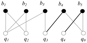
Solution: Find the free bidder b1.
Let consider bidder b1:
.

Consider bidder b2:
.
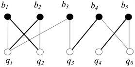
Consider bidder b3:
.
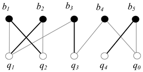
Now consider on bidder b4:
.
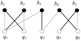
Thus the maximum matching for the bipartite graph is:
.
4. Pricing Algorithm of Matched Items
Algorithm: Pricing of maximized items
input W = maxwi \\Obtaining revenue
input
\\ allocated bidders in the auction
input
\\ the price of demanded items
for all
do
Winner = 0;
; \\ duration of time
;
If
then \\ (p,
) now is an equilibrium
Winner = 1;
;
For all
do \\decreasing the items
t++;
winner = 0;
else
;
Break;
Output
5. The Main Results
In our dynamic auction market let B be the set of bidders and N set of the items in the market (B, N, c, v), c is the reservation price of items in Set N and V is a private value for each bidder who bids items in the auction.
Theorem 4.1: let p be the maximum competitive price vector obtained from the auction mechanism and let y be any other competitive price.
Proof: By contradiction, suppose
. At stage t = 1 of the auction
so
.
(1)
Define
. If bidders claim that
. then chose q in
and if
then bidder claim
and chose q in
. That means bidder b prefers item q to j if
b prefer q to j at a price
because
. but when
and
bidder b chose q at a price of y. if
then bidder b prefer item q at least as well item j at price
. but when
again,
then bidder b prefer item q at price y . So in y price there is no over-demanded items.
(2)
where
. So
which is
is over-demanded.
Theorem 4.2: let p be the maximum competitive price then there is a feasible allocation
such that
is an equilibrium.
Proof: let π an assignment to price p where item j is over-demanded. if
is not an equilibrium then
. For this purpose we propose Maximum matching in bipartite graph to eliminate over-demanded items.
Step 1: The auctioneer announces the upper bound price
and bidders demand their valuation at these prices in which
, then the auctioneer decrease the price without changing the price of the other items. this step repeats until each item has at least one demand.
![]()
Table 1. Bidders valuation on the items.
Step t + 1: In this step the price of items that are demanded are
and some of the other items including the dummy are
. The auctioneer stops the auction until every bidder
get one item. Otherwise (Hall’s Theorem) which states that some of the other bidders demand over-priced items then the auctioneer chooses the minimal over-priced item and decrease the price without any change of the other items.
This example illustrates our mechanism.
Example: Let
,
and
. the bidders revealed value go to Table 1. The auctioneer announces the upper bound price
. in which we can also say Maximum Matching price M.
Step p (t): auctioneer announces price
, bidders require items, because the price is expensive, no bidders are reasonably priced, so the auctioneer lowers the price of all items unit untill p (11, 8, 6, 0), so bidder b2 demand item 2 and 3 and bidder b4 demand item 2 and 3 then the auctioneer decrease the price of item 1 without changing the price of the other items until p (9, 8, 6, 0) then the bidders b2 demand item 2 and 3 and bidder b3 demands item 1, 3 and q0. the auctioneer finds a minimal over-priced set
then decreases the price of three items by one unit. then go Step 2.
Step 2
Bidders b2 demands item 2 and 3 and bidder b2 demands item 1, 2 and 3 and bidder b3 demands item 1, 3 and q0 and bidder b4 demands item 2 and q0. then the auctioneer decides to allocate the items to their bidders with a three choice of outcome.
and
,
and
,
and
,
and
and
and
,
and
.
6. Conclusion and Discussion
In a dynamic market auction, the trading process is decentralized and it is modeled for pairwise meetings. The COVID-19 outbreak since December 2019 has attracted more attention which has turned the PPE companies to feature a temporary excess demand and supply without affecting prices extremely to agent levels. Following the presented model, the equilibrium price was above zero. The equilibrium price has been a non-market-clearing in the fact that there is a shown excess demand which has been consistent with the price above the buyer’s reservation level (Allevi et al., 2012). This is brought about by the recession and trading frictions.
The significant conclusion which can be made from this research and response to the dynamic market auction under the protective equipment on COVID-19 is: the non-market-clearing price phenomenon can never be replaced by the new feature.
The new feature towards the excess demand in the dynamic market auction shows that it is translated into instantaneous bidding competition. The phenomenon is dependent on how the used technology distributes the sellers among the buyers so that the equilibrium can be achieved. The significance of the degree of heterogeneity of the buyer’s valuations as captured by the distributions is relative to the cost of time captured. The instantaneous bidding competition is not significant if the cost of time is small and relative to the heterogeneity of valuations. This aspect means that the environment is similar to that of pairwise meetings models and may lead to non-market-clearing issue. In disequilibrium macroeconomics, companies observe their own sales to set their competing non-market clearing prices. If their own sales provide additional information, and this information is valuable, then companies can use non-market clearing prices to get this information.
In the market auction, the competition for the new features of ultra-demand is transformed into the technology of real-time bidding. If time costs are heterogeneous relative to costs, then timely forecasting of competition is not important. Therefore, excess demand is the main problem that leads to the imbalance of the current equilibrium, and it may take some time to achieve equilibrium. The results presented here show that for the bid drop is small enough, our mechanism is through matching the highest price equilibrium for the bidder who needs it most. Nonetheless, our results only give linear surpluses here. The analysis of more general quotas is still a problem for future investigations, and we hope that the model focused here will help build understand.