Efficient BTCS + CTCS Finite Difference Scheme for General Linear Second Order PDE

Gueye Serigne Bira, Mbow Cheikh, Diagana Mouhamed Fadel

Département de Physique, Faculté des Sciences et Techniques, Université Cheikh Anta Diop, Dakar-Fann, Sénégal.

DOI: 10.4236/jemaa.2021.1310010                

Abstract

This work deals with a second order linear general equation with partial derivatives for a two-variable function. It covers a wide range of applications. This equation is solved with a finite difference hybrid method: BTCS + CTCS. This scheme is simple, precise, and economical in terms of time and space occupancy in memory.

Keywords

Finite Difference, BCTS + CTCS, Usmani’s Algorithm, Tridiagonal Matrix, Telegraph Equation

1. Introduction

We are interested in the following second order linear Partial Differential Equation (PDE):

$\begin{array}{l}A\left(x\mathrm{,}t\right)\frac{{\partial }^2\Phi }{\partial x^2}+B\left(x\mathrm{,}t\right)\frac{{\partial }^2\Phi }{\partial x\partial t}+C\left(x\mathrm{,}t\right)\frac{{\partial }^2\Phi }{\partial t^2}+D\left(x\mathrm{,}t\right)\frac{\partial \Phi }{\partial x}\\ +E\left(x\mathrm{,}t\right)\frac{\partial \Phi }{\partial t}+F\left(x\mathrm{,}t\right)\Phi =g\left(x\mathrm{,}t\right)\mathrm{<mo>\; ;\; </mo>}\end{array}$ (1)

where $\Phi$ designates an scalar function depending on the variables x and t. Usually x states for the space variable and t for the time. The Equation (1) can be brought in the following form:

${\displaystyle \underset{\mu =0}{\overset{2}{\sum }}}{\displaystyle \underset{\nu =0}{\overset{2-\mu }{\sum }}}{A}_{\mu }^{\nu }\left(x,t\right)\frac{{\partial }^{\mu }{\partial }^{\nu }\Phi }{\partial x^{\mu }\partial t^{\nu }}=g\left(x,t\right)\cdot$ (2)

The resolution of such an equation presents a great interest, because it governs several phenomenas in physics, chemistry, mathematics, economy, etc. [1]. It is a general form that deals with:

· Elliptic equations: It treats the Poisson equation which describes electrostatic and magnetostatic phenomenas, flow of perfect incompressible fluids, vortex and viscous incompressible flow, filtration of fluids through porous materials, etc. It concerns also the Euler-Tricomi equation that allows the study of transonic flow.

· Parabolic equations: It handles problems governed by the extended diffusion equation or the Diffusion Advection Reaction equation (of concentration, matter, temperature or electromagnetic field) or the BlackScholes equation in mathematical finance [2] [3].

· Hyperbolic equation: Equations such the extended complete wave equation and the extended complete telegraph equation are contained in (1). These two equations have important applications in electromagnetic and telecommunications [4] [5] [6] [7].

We propose to solve this equation with a simple, accurate and efficient method, by reducing the costs in time, memory space, and method’s heaviness. We aim at a good compromise between simplicity and result accuracy.

So, we will first, formulate the problem. Then, we choose a hybrid approximation scheme, using two finite differences approaches: Backward Time Centered Space (BTCS) and Centered Time Centered Space (CTCS) [8] [9] [10]. This heterogeneous scheme has the advantages of both. The first method BTCS is implicit and the second one is explicit. With their superposition, the resulting method becomes implicit. Therefore, we will use different methods for processing the matrices that result from the discretization. These methods are the algorithm of Usmani [11], which inverts any regular tridiagonal matrix directly; and the algorithm of Thomas which inverts a diagonal dominant tridiagonal matrix using the Right Hand Side (RHS) of the equation.

Subsequently, we will treat numerical experimentation to validate our proposed method. Finally, we discuss the results and give outlook for further work.

2. Problem Formulation and Meshing

We consider a scalar function $\Phi =\Phi \left(x\mathrm{,}t\right)$ which depends on the real variables x and t. This function satisfies the partial differential Equation (3) with the given conditions.

$\{\begin{array}{l}A{\Phi }_{xx}+B{\Phi }_{xt}+C{\Phi }_{tt}+D{\Phi }_x+E{\Phi }_t+F\Phi =g,\left(x,t\right)\in \left]0,L\right[\times \left]0,\infty \right[\\ \Phi \left(x,0\right)=f_0\left(x\right),{\Phi }_t\left(x,0\right)=f_1\left(x\right),x\in \left]0,L\right[\\ \Phi \left(0,t\right)=g_0\left(t\right),\Phi \left(L,t\right)=g_L\left(t\right),t\in \left]0,\infty \right[\end{array}$ (3)

Here, The coefficients A, B, C, D, E and F are constant or known functions depending on the variables x and t. L is a real constant. The function $g=g\left(x\mathrm{,}t\right)$ is a known excitation. The functions $f_0\left(x\right)$, $f_1\left(x\right)$, $g_0\left(t\right)$ and $g_L\left(t\right)$ have been also given.

The following mesh has been considered: the spatial interval $\left[\mathrm{0,}L\right]$ is discretized in $N_x+2$ points $x_i=i\cdot \Delta x,i=0,1,2,\cdots ,N_x+1$, with $\Delta x=h=L\left(N_x+1\right)$. The considered instants are: $t_n=n\cdot \Delta t$. The time step is $\Delta t=k$ and must be sufficiently small to allow a good, accurate and efficient resolution of the problem. An approximated value of $\Phi$ is to be found at point $\left(x_i\mathrm{,}{t}_n\right)$ : $\Phi \left(x_i\mathrm{,}{t}_n\right)={\Phi }_i^n$. We define: $g\left(x_i\mathrm{,}{t}_n\right)=g_i^n$, $g_0\left(t_n\right)=g_0^n$, $g_L\left(t_n\right)=g_L^n$, $f_0\left(x_i\right)=f_0{}_i$ and $f_1\left(x_i\right)=f_1{}_i$. It holds: $A\left(x_i\mathrm{,}{t}_n\right)=A_i^n$, $B\left(x_i\mathrm{,}{t}_n\right)=B_i^n$, $C\left(x_i\mathrm{,}{t}_n\right)=C_i^n$, $D\left(x_i\mathrm{,}{t}_n\right)=D_i^n$, $E\left(x_i\mathrm{,}{t}_n\right)=E_i^n$ and $F\left(x_i\mathrm{,}{t}_n\right)=F_i^n$.

3. Schema BTCS + CTCS

We consider the Finite Difference method in Time Domain (FDTD); more precisely the two schemes: BTCS and CTCS [8] [9] [10]. Then, we superpose the two approaches in order to obtain a better approximation of the solution of the treated differential equation. In this way we combine the advantages of the two schemes. As one can remark, these two schemes have the same spatial discretization (Centered Space CS). Thus, we have for the derivative in x direction the following approximations:

$\begin{array}{l}\left(\frac{\partial \Phi }{\partial x}\right)\left(x_i\mathrm{,}{t}_n\right)=\frac{{\Phi }_{i+1}^n-{\Phi }_{i-1}^n}{2h}+O\left(h^2\right)\mathrm{,}\\ \left(\frac{{\partial }^2\Phi }{\partial x^2}\right)\left(x_i\mathrm{,}{t}_n\right)=\frac{{\Phi }_{i-1}^n-2{\Phi }_i^n+{\Phi }_{i+1}^n}{h^2}+O\left(h^2\right)\mathrm{,}i=\mathrm{1,2,3,}\cdots \mathrm{,}{N}_x\mathrm{.}\end{array}$ (4)

For the BTCS scheme, we get the first and second order backward time derivatives, for $t_n>0$ :

$\begin{array}{l}\left(\frac{\partial \Phi }{\partial t}\right)\left(x_i\mathrm{,}{t}_n\right)=\frac{{\Phi }_i^n-{\Phi }_i^{n-1}}{k}+O\left(k\right)\mathrm{,}\\ \left(\frac{{\partial }^2\Phi }{\partial t^2}\right)\left(x_i\mathrm{,}{t}_n\right)=\frac{{\Phi }_i^n-2{\Phi }_i^{n-1}+{\Phi }_i^{n-2}}{k^2}+O\left(k\right)\mathrm{,}i=\mathrm{1,2,3,}\cdots \mathrm{,}{N}_x\mathrm{.}\end{array}$ (5)

Combining the Equations (3)-(5), one gets:

$\begin{array}{l}\underset{:=c_i^b}{\underset{︸}{\left(A_i^n-\frac{h}{2k}{B}_i^n-\frac{h}{2}{D}_i^n\right)}}{\Phi }_{i-1}^n+\underset{:=d_i^b}{\underset{︸}{\left(-2A_i^n+\frac{h^2}{k^2}{C}_i^n+\frac{h^2}{k}{E}_i^n+h^2{F}_i^n\right)}}{\Phi }_i^n\\ +\underset{:=e_i^b}{\underset{︸}{\left(A_i^n+\frac{h}{2k}{B}_i^n+\frac{h}{2}{D}_i^n\right)}}{\Phi }_{i+1}^n,\\ =\underset{:=-{c^{\prime }}_i^b}{\underset{︸}{\left(-\frac{h}{2k}{B}_i^n\right)}}{\Phi }_{i-1}^{n-1}+\underset{:={d^{\prime }}_i^b}{\underset{︸}{\left(2\frac{h^2}{k^2}{C}_i^n+\frac{h^2}{k}{E}_i^n\right)}}{\Phi }_i^{n-1}+\underset{:={e^{\prime }}_i^b}{\underset{︸}{\left(\frac{h}{2k}{B}_i^n\right)}}{\Phi }_{i+1}^{n-1}\\ +\underset{:=b_i^b}{\underset{︸}{\left(-\frac{h^2}{k^2}{C}_i^n\right)}}{\Phi }_i^{n-2}+h^2{g}_i^n,i=2,3,\cdots ,N_x-1;n\ge 1.\end{array}$ (6)

With the CTCS scheme, we have the following first and second order derivatives, for $t_n>0$ :

$\begin{array}{l}\left(\frac{\partial \Phi }{\partial t}\right)\left(x_i,t_n\right)=\frac{{\Phi }_i^{n+1}-{\Phi }_i^{n-1}}{2k}+O\left(k^2\right),\\ \left(\frac{{\partial }^2\Phi }{\partial t^2}\right)\left(x_i,t_n\right)=\frac{{\Phi }_i^{n-1}-2{\Phi }_i^n+{\Phi }_i^{n+1}}{k^2}+O\left(k^2\right),i=1,2,3,\cdots ,N_x.\end{array}$ (7)

Associating the Equations (3), (4), and (7); one gets:

$\begin{array}{l}\underset{:=c_i^c}{\underset{︸}{\left(-\frac{h}{4k}{B}_i^{n-1}\right)}}{\Phi }_{i-1}^n+\underset{:=d_i^c}{\underset{︸}{\left(\frac{h^2}{k^2}{C}_i^{n-1}+\frac{h^2}{2k}{E}_i^{n-1}\right)}}{\Phi }_i^n+\underset{:=e_i^c}{\underset{︸}{\left(\frac{h}{4k}{B}_i^{n-1}\right)}}{\Phi }_{i+1}^n\\ =\underset{:={c^{\prime }}_i^c}{\underset{︸}{\left(-A_i^{n-1}+\frac{h}{2}{D}_i^{n-1}\right)}}{\Phi }_{i-1}^{n-1}+\underset{:={d^{\prime }}_i^c}{\underset{︸}{\left(2A_i^{n-1}+2\frac{h^2}{k^2}{C}_i^{n-1}-h^2{F}_i^{n-1}\right)}}{\Phi }_i^{n-1}\\ +\underset{:={e^{\prime }}_i^c}{\underset{︸}{\left(-A_i^{n-1}-\frac{h}{2}{D}_i^{n-1}\right)}}{\Phi }_{i+1}^{n-1}+\underset{:=-a_i^c}{\underset{︸}{\left(-\frac{h}{4k}{B}_i^{n-1}\right)}}{\Phi }_{i-1}^{n-2}+\underset{:=b_i^c}{\underset{︸}{\left(-\frac{h^2}{k^2}{C}_i^{n-1}+\frac{h^2}{2k}{E}_i^{n-1}\right)}}{\Phi }_i^{n-2}\\ +\underset{:=a_i^c}{\underset{︸}{\left(\frac{h}{4k}{B}_i^{n-1}\right)}}{\Phi }_{i+1}^{n-2}+h^2{g}_i^{n-1},i=2,\cdots ,N_x-1;n\ge 2.\end{array}$ (8)

We define $c_i=c_i^b+c_i^c$, $d_i=d_i^b+d_i^c$, $e_i=e_i^b+e_i^c$, ${c^{\prime }}_i={c^{\prime }}_i^b+{c^{\prime }}_i^c$, ${d^{\prime }}_i={d^{\prime }}_i^b+{d^{\prime }}_i^c$, ${e^{\prime }}_i={e^{\prime }}_i^b+{e^{\prime }}_i^c$, $a_i=0+a_i^c$ and $b_i=b_i^b+b_i^c$ ; for $i=1,2,3,\cdots ,N_x;n\ge 1$. Thus, we obtain the following matrix equation, considering the mesh points $x_1$ and $x_{N_x}$ :

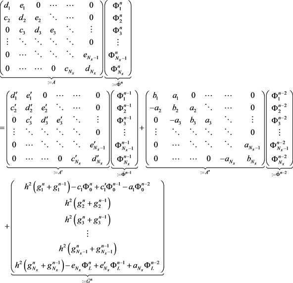(9)

This previous equation is equivalent to:

${\left(A\right)}^n{\stackrel{\to }{\Phi }}^n=\underset{:={\stackrel{\to }{H}}^n}{\underset{︸}{{\left(A^{\prime }\right)}^n{\stackrel{\to }{\Phi }}^{n-1}+{\left(A^{″}\right)}^n{\stackrel{\to }{\Phi }}^{n-2}+{\stackrel{\to }{G}}^n}},n\ge 2,$ (10)

with

${\Phi }_i^{-1}=\left({\Phi }_i^0-k{\Phi }_t{}_i^0\right)\text{and}{\Phi }_i^1=\left(2k{\Phi }_t{}_i^0+{\Phi }_i^{-1}\right)\cdot$ (11)

So, we will discuss the inversion methods of the matrix ${\left(A\right)}^n$, which permits to get the solution ${\stackrel{\to }{\Phi }}^n$.

4. General Solution

An important discussion is to be done with respect to Equation (9), particularly concerning the matrix ${\left(A\right)}^n$. Principally, this matrix must be inverted for each time $t_n$ in order to get the solution at this time: ${\stackrel{\to }{\Phi }}^n$. But, if the coefficients of Equation (1) do not dependent on the time ${\left(A\right)}^n=\left(A\right)$ then one and exactly one inversion is sufficient.

The algorithm of Thomas can be used for the inversion (see Appendix). With this method, we do not have an idea about the regularity of the matrix. But, it is clear that if the tridiagonal matrix ${\left(A\right)}^n$ is diagonal dominant then it is regular. Of course, this property is sufficient but not necessary for the regularity.

We prefer an inversion with the Usmani’s algorithm [11], which is a general and stable method. It allows a direct inversion that does not use the right hand side ( ${\stackrel{\to }{H}}^n$ ) in the inversion process; contrarily to the algorithm of Thomas. Usmani has presented a direct and exact method to invert a tridiagonal regular matrix [11].

We can apply it for ${\left(A\right)}^n$, defining:

$\begin{array}{l}{\theta }_0=1,{\theta }_1=d_1,{\theta }_{N_x+1}=0\text{and}{\theta }_i=d_i{\theta }_{i-1}-c_i{e}_{i-1}{\theta }_{i-2},i=2,3,\cdots ,N_x,\\ \text{and}{\eta }_{N_x+1}=1,{\eta }_{N_x}=d_{N_x},{\eta }_0=0\text{and}\\ {\eta }_i=d_i{\eta }_{i+1}-c_{i+1}{e}_i{\eta }_{i+2},i=N_x-1,N_x-2,\cdots ,2,1\end{array}$

Then, the coefficients of the inverted matrix ${\left(B\right)}^n$ are obtained with:

$b_{ij}=\{\begin{array}{ll}{\left(-1\right)}^{i+j}\cdot {\displaystyle \underset{l=i}{\overset{j-1}{\prod }}}{e}_l\cdot \frac{{\theta }_{i-1}\cdot {\eta }_{j+1}}{{\theta }_{N_x}}\hfill & i<j\hfill \\ \frac{{\theta }_{i-1}\cdot {\eta }_{i+1}}{{\theta }_{N_x}}\hfill & i=j\hfill \\ {\left(-1\right)}^{i+j}\cdot {\displaystyle \underset{l=j}{\overset{i-1}{\prod }}}{c}_l\cdot \frac{{\theta }_{j-1}\cdot {\eta }_{i+1}}{{\theta }_{N_x}}\hfill & i>j\hfill \end{array}$ (12)

We get the solution:

${\stackrel{\to }{\Phi }}^n={\left(B\right)}^n\times {\stackrel{\to }{H}}^n\mathrm{.}$ (13)

The solution ${\Phi }_i^n$, at point $x_i$ and time $t_n$, is given by a simple matrix- vector multiplication:

${\Phi }_i^n={\displaystyle \underset{j=1}{\overset{N_x}{\sum }}}{b}_{ij}\cdot {\underset{\_}{H}}_j^n,i=1,2,\cdots ,N_x,n\ge 2.$ (14)

5. Solution for Time-Depending Coefficients

In the case that the coefficients of Equation (1) do not dependent on the space: $A=A\left(t\right)$, $B=B\left(t\right)$, $C=C\left(t\right)$, $D=D\left(t\right)$, $E=E\left(t\right)$ and $F=F\left(t\right)$ ; then the matrix (A) dependent only on the time. Its coefficients are constant at a fixed time $t_n$. The formula of the invert matrix ${\left(B\right)}^n$ can be simplified [12] [13] [14]:

Defining a real number $\Delta$ and a complex number $\theta$ in following manner:

$\Delta =d^2-4ec\text{and}\theta =\text{atanh}\left(\frac{\sqrt{\Delta }}{d}\right).$ (15)

we get ${\left|A\right|}_i,i=1,2,\cdots ,N_x$, which is the determinant of the submatrix of order i of (A); and which is of dimension ( $i\times i$ ). In the case, where $e\cdot c=0$, the determinant of the matrix (A) is: ${\left|A\right|}_{N_x}=d^{N_x}$

One can verify that this determinant, for $e\cdot c\ne 0$, is given by the following relations [12] [13] [14]:

${\left|A\right|}_{N_x}=\{\begin{array}{l}\frac{1}{\sqrt{\Delta }}\left\{{\left[\frac{d+\sqrt{\Delta }}{2}\right]}^{N_x+1}-{\left[\frac{d-\sqrt{\Delta }}{2}\right]}^{N_x+1}\right\}={\left(\pm \mathrm{sgn}\left(d\right)\sqrt{\left|ec\right|}\right)}^{N_x}\frac{\sinh \left(\left(N_x+1\right)\theta \right)}{\sinh \left(\theta \right)},d\ne \pm 2\sqrt{ec}\\ {\left(\pm \sqrt{\left|ec\right|}\right)}^{N_x}\left(N_x+1\right),d=\pm 2\sqrt{\left|ec\right|}\end{array}$ (16)

The inverted matrix (B) exists when d is different of one of the following values [14]:

$d_l=2\sqrt{ec}\cos \left(\frac{l\pi }{N_x+1}\right),l=1,2,\cdots ,N_x.$ (17)

Outside these values of $d_l$, the matrix (A) is regular and its inverts (B) is given by the following formula:

$b_{ij}=\{\begin{array}{ll}{\left(-1\right)}^{i+j}\cdot e^{j-i}\cdot \frac{{\left|A\right|}_{i-1}\cdot {\left|A\right|}_{N_x-j}}{{\left|A\right|}_{N_x}}\hfill & i\le j\hfill \\ {\left(-1\right)}^{i+j}\cdot c^{i-j}\cdot \frac{{\left|A\right|}_{j-1}\cdot {\left|A\right|}_{N_x-i}}{{\left|A\right|}_{N_x}}\hfill & i>j\hfill \end{array},1\le i,j\le N_x$ (18)

6. Numerical Verification

For the numerical verification, we choose the equation of telegraph equation, which has been treated by several authors [4] [5] [6] [7]. We compare our results with those obtained by [4].

The following problem treated by [4] was considered and our method was applied:

$\{\begin{array}{l}-{\Phi }_{xx}\left(x,t\right)+{\Phi }_{tt}\left(x,t\right)+2\alpha {\Phi }_t\left(x,t\right)+{\beta }^2\Phi \left(x,t\right)=g\left(x,t\right),\left(x,t\right)\in \left]0,\pi \right[\times \left]0,\infty \right[\\ \Phi \left(x,0\right)=f_0\left(x\right)=\sin \left(x\right),{\Phi }_t\left(x,0\right)=f_1\left(x\right)=-\sin \left(x\right),x\in \left]0,\pi \right[\\ \Phi \left(0,t\right)=g_0\left(t\right)=0,\Phi \left(\pi ,t\right)=g_L\left(t\right)=0,t\in \left]0,\infty \right[\end{array}$ (19)

By choosing dx = 0.02 and dt = 0.001, the following results were obtained, showing the $L_{\infty }$ and $L_2$ errors:

The results are very satisfactory because our method is not heavy and leads to a precise solution. Compared to the one used in [4], it could be said to be less precise. But it should be emphasized that the method, used in [4], is a Cubic B-splines collocation method, which is expensive in calculation. On the other hand, we used the finite difference method.

7. Conclusions

In this work, a method of solving a general linear partial differential equation has been presented. The finite difference hybrid approach (BTCS + FTCS) that has been used is simple, accurate and efficient; and is economical in terms of calculation and occupancy of the memory space.

This study can allow numerous applications of this method to several phenomena of the sciences and techniques governed by this equation. In addition, other methods could be explored to improve performance.

Appendix

For a resolution of Equation (10) with the algorithm of Thomas, the vector $\stackrel{\to }{\alpha }$, $\stackrel{\to }{\gamma }$, and $\stackrel{\to }{r}$ can be introduced, in order to proceed to a forward elimination. Then the solutions are obtained by backward restitution. This algorithm is presented below.

Conflicts of Interest

The authors declare no conflicts of interest regarding the publication of this paper.

References

[1]	Kuneš, J. (2012) Similarity and Modeling in Science and Engineering. Cambridge International Science Publishing, 131-141.
[2]	Gurarslan, G., Karahan, H., Alkaya, D., Sari, M. and Yasar, M. (2013) Numerical Solution of Advection-Diffusion Equation Using a Sixth-Order Compact Finite Difference Method. Mathematical Problems in Engineering, 2013, Article ID: 672936. https://doi.org/10.1155/2013/672936
[3]	Crank, J. and Nicolson, P. (1947) A Practical Method for Numerical Evaluation of Solutions of Partial Differential Equations of the Heat Conduction Type. Proceedings of the Cambridge Philosophical Society, 43, 50-67. https://doi.org/10.1017/S0305004100023197
[4]	Mittal, R.C. and Bhatia, R. (2013) Numerical Solution of Second Order One Dimensional Hyperbolic Telegraph Equation by Cubic B-Spline Collocation Method. Applied Mathematics and Computation, 220, 496-506. https://doi.org/10.1016/j.amc.2013.05.081
[5]	Inc, M., Akgül, A. and Kiliüman, A. (2013) Numerical Solutions of the Second-Order One-Dimensional Telegraph Equation Based on Reproducing Kernel Hilbert Space Method. Abstract and Applied Analysis, 2013, Article ID: 768963. https://doi.org/10.1155/2013/768963
[6]	Pandit, S., Kumar, M. and Tiwari, S. (2015) Numerical Simulation of Second-Order Hyperbolic Telegraph Type Equations with Variable Coefficients. Computer Physics Communications, 187, 83-90. https://doi.org/10.1016/j.cpc.2014.10.013
[7]	Lakestani, M. and Saray, B.N. (2010) Numerical Solution of Telegraph Equation Using Interpolating Scaling Functions. Computers and Mathematics with Applications, 60, 1964-1972. https://doi.org/10.1016/j.camwa.2010.07.030
[8]	Sadiku Matthew, N.O. (2000) Numerical Techniques in Electromagnetics. 2nd Edition, CRC Press, Boca Raton, 15-19. https://doi.org/10.1201/9781420058277
[9]	Engeln-Muellges, G. and Reutter, F. (1991) Formelsammlung zur Numerischen Mathematik mit QuickBasic-Programmen. Dritte Auflage, BI-Wissenchaftsverlag, 472-481.
[10]	Conte, S.D. and de Boor, C. (1981) Elementary Numerical Analysis: An Algorithmic Approach. 3rd Edition, McGraw-Hill, New York, 153-157.
[11]	Usmani, R.A. (1994) Inversion of a Tridiagonal Jacobi Matrix. Linear Algebra and Its Applications, 212-213, 413-414. https://doi.org/10.1016/0024-3795(94)90414-6
[12]	Gueye, S.B. (2014) Semi-Analytical Solution of the 1D Helmholtz Equation, Obtained from Inversion of Symmetric Tridiagonal Matrix. Journal of Electromagnetic Analysis and Applications, 6, 425-438. https://doi.org/10.4236/jemaa.2014.614044
[13]	Hu, G.Y. and O’Connell, R.F. (1996) Analytical Inversion of Symmetric Tridiagonal Matrices. Journal of Physics A, 29, 1511-1513. https://doi.org/10.1088/0305-4470/29/7/020
[14]	da Fonseca, C.M. and Petronilho, J. (2001) Explicit Inverses of Some Tridiagonal Matrices. Linear Algebra and Its Applications, 325, 7-21.