Rational Points on Genus 3 Real Hyperelliptic Curves

Brice M. Miayoka, Regis F. Babindamana, Basile G. R. Bossoto

Faculté Des Sciences et Techniques, Université Marien Ngouabi, Brazzaville, Congo.

DOI: 10.4236/ojdm.2021.114008                

Abstract

We compute rational points on real hyperelliptic curves of genus 3 defined on whose Jacobian have Mordell-Weil rank r=0. We present an implementation in sagemath of an algorithm which describes the birational transformation of real hyperelliptic curves into imaginary hyperelliptic curves and the Chabauty-Coleman method to find C (). We run the algorithms in Sage on 47 real hyperelliptic curves of genus 3.

Keywords

Hyperelliptic Curve, Jacobian, Coleman Integration, Rational Point

1. Introduction

Let C be a hyperelliptic curve of the genus $g\ge 2$ defined on $\mathbb{Q}$. The Mordell conjecture proved by Fattings, gives that the set of rational points $C\left(\mathbb{Q}\right)$ is finite. The hyperelliptic curves can be subdivided into two types: those with real models and those with imaginary models. Our objective is to compute the rational points in the case of real hyperelliptic curves of genus 3 whose Jacobian have a Mordel-Weil rank equal to 0. This fits into the particular case where $r<g$ has been considered by Chabauty and the techniques developed by Coleman in 1980 [1], allow us to use the p-adic integration to explicitly computation the set of rational points [2].

The AMS classification: MSC2020, 14G05, 11G30.

Although there is an algorithm by Jennifer Balakrishnan computing Coleman integrals in the case of real hyperelliptic curves in [3], this one is unfortunately not available in Sage. We then use the birational transformation of real hyperelliptic curves into imaginary hyperelliptic curves, because in the latter case, Balakrishnan, Bradshaw and Kedlaya described and implemented in Sage the explicit computation of Coleman integrals on imaginary hyperelliptic curves [4]. We start with an overview of hyperelliptic curves and the transition from a real hyperelliptic curve to an imaginary hyperelliptic curve in Section 1. In Section 2, we recall the Chabauty-Coleman method and explicit Coleman integration. In Section 3, we describe our algorithm, which is subdivided into three sub-algorithms: the first one that transforms a real curve to an imaginary curve; the second computes the set of rational points of the imaginary hyperelliptic curve found in Algorithm 3. Algorithm 4 is this of Maria Inés de Frutos Fernaandez and Sachi Hashimoto in [5] and its implementation in [6]. To the latter, we added a function allowing it to take the hyperelliptic curves of genus 3 and of rank 0 given by non-monic polynomials. Finally, the third algorithm constructs the rational points of the curve C which is real hyperelliptic from the rational points of the imaginary hyperelliptic curve birationally equivalent to C. In Section 4, we present the results obtained on a list of curves taken from the database of hyperelliptic curves of genus 3 [7].

2. Background on Hyperelliptic Curves

In this section we recall the definition of hyperelliptic curves, the different types of hyperelliptic curves and how to pass from a real hyperelliptic curve to an imaginary hyperelliptic curve. For more detail in this section, we refer the reader to [8] [9]. A hyperelliptic curve of genus $g\ge 2$ over $\mathbb{Q}$ is defined by an equation:

$y^2=f\left(x\right)$ (1)

where f is a polynomial of $\mathbb{Q}\left[x\right]$ of degree $2g+2$ or $2g+1$. This defines a smooth irreducible algebraic curve in the affine plane. Considering its smooth projective model which is obtained by adding one or two points at infinity, we distinguish two types of hyperelliptic curves which differ by the number of rational points at infinity:

- Real hyperelliptic curves: they are those which have two points at infinity. In this case, the polynomial f is of degree $2g+2$ ;

- Imaginary hyprelliptic curves: they are those which have a one point at infinity. In this case, the polynomial f is of degree $2g+1$.

In this article, we are interested in real hyperelliptic curves.

A real hyperelliptic curve C of genus g over $\mathbb{Q}$ is defined by an absolutely irreducible equation of the form:

$y^2=f\left(x\right)=f_{2g+2}{x}^{2g+2}+f_{2g+1}{x}^{2g+1}+f_{2g}{x}^{2g}+f_{2g-1}{x}^{2g-1}+\cdots +f_0$ (2)

where $f_{2g+2}\ne 0$. The two points at infinity correspond to the two square roots of the leading coefficient of f. These points are rational if and only if this leading coefficient is a square, so that its square roots are rational numbers.

Let us soppose that $f_{2g+2}$ is a non-zero square in $\mathbb{Q}$. We set $f_{2g+2}=s^2$. The points at infinity of C are given in projective coordinates by ${\infty }_1=\left(\mathrm{1\; <mo>\; :\; </mo>}s\mathrm{<mo>\; :\; </mo>0}\right)$ and ${\infty }_2=\left(\mathrm{1\; <mo>\; :\; </mo>}-s\mathrm{<mo>\; :\; </mo>0}\right)$, which are rational [9].

The set of rational points on C denoted by $C\left(\mathbb{Q}\right)$, is defined by:

$C\left(\mathbb{Q}\right)=\left\{\left(x\mathrm{,}y\right){\mathbb{Q}}^2|y^2=f\left(x\right)\right\}\cup \left\{{\infty }_1\mathrm{,}{\infty }_2\right\}$

Let C be a real hyperelliptic curve of genus g over $\mathbb{Q}$ with equation $y^2=f\left(x\right)$. If there exists a ramified prime divisor of degree 1 in $\mathbb{Q}$ of C, then the curve C is birationally equivalent to an imaginary hyperelliptic curve $C^{\prime }\mathrm{<mo>\; :\; </mo>}{y^{\prime }}^2=f^{\prime }\left(x^{\prime }\right)$ of genus g. Indeed, if we denote $P=\left(a\mathrm{,}b\right)$ a rational point of the curve C such that P is equal to its image under the hyperelliptic involution $\iota \left(P\right)=\left(a\mathrm{,}-b\right)$ i.e.: that $2b=0$, then P is said to be ramified and in this case the divisor $D=P-{\infty }_1$ is the ramified prime divisor, then we can make the following change of variable:

$x=\frac{1+a{x}^{\prime }}{x^{\prime }}\text{and}y=\frac{y^{\prime }}{{x^{\prime }}^{g+1}}-b$ (3)

In the equation of C, we thus find the equation of $C^{\prime }$.

Therefore P is ramified if $b=0$. By substituting a and $b=0$ in the equation of C, we get $f\left(a\right)=0$. We conclude that if the polynomial $f\left(x\right)$ has at least one root in $\mathbb{Q}$, then the real hyperelliptic curve of equation $y^2=f\left(x\right)$ admits at least one rational ramified point and therefore it is birationally equivalent to an imaginary hyperelliptic curve via the change of variables below.

We are interested in real hyperelliptic curves of genus 3 having at least one rational point of ramification and whose Jacobians have Mordell-Weil rank 0.

3. Background Chabauty-Coleman Method and Coleman Integration

In this section we recall the Chabauty-Coleman method used to compute the rartional points in part 2 of our algorithm. We also give a brief reminder on Coleman integrals. For more details see [10].

3.1. Chabauty-Coleman Method

Let C be a smooth projective curve over the rational numbers of genus at least 2. From the work of Faltings, we know that $C\left(\mathbb{Q}\right)$ is finite, but the proof of Faltings does not explicitly give the set $C\left(\mathbb{Q}\right)$. However, before Faltings’ work, Chabauty considered the following configuration. Let p be a prime number and $P\in C\left({\mathbb{Q}}_p\right)$. We consider the following inclusion:

${\iota }_P\mathrm{<mo>\; :\; </mo>}C\to J\mathrm{,}Q\to \left[Q-P\right]$.

Let $\overline{J\left(\mathbb{Q}\right)}$ be the p-adic closure of $J\left(\mathbb{Q}\right)$ and define $C\left({\mathbb{Q}}_p\right)\cap \overline{J\left(\mathbb{Q}\right)}={\iota }_P\left(C\left({\mathbb{Q}}_p\right)\right)\cap \overline{J\left(\mathbb{Q}\right)}$. Chabauty proved the following case of Mordell’s conjecture:

Theorem 2.1. Let $C/\mathbb{Q}$ be a curve of genus $g\ge 2$ such that the Mordell-Weil the rank of the Jacobian J of C over Q is less than g, and let p be a prime number, then $C\left({\mathbb{Q}}_p\right)\cap \overline{J\left(\mathbb{Q}\right)}$ is finite.

Chabauty’s result was then reinterpreted and made effective by Coleman, who showed what follows:

Theorem 2.2. Let C be as above and suppose that p is a prime number of good reduction for C. If $p>2g$ , then:

$\#C\left(\mathbb{Q}\right)\le \#C\left({\mathbb{F}}_p\right)+2g-2$.

The Chabauty-Coleman method uses the theory of p-adic integrations on curves to construct the p-adic integrals of 1-forms on $C\left({\mathbb{Q}}_p\right)$ which vanish on $C\left(\mathbb{Q}\right)$ and which allow in practice to explain the set of rational points which are contained in the intersection of the set of zeros of the integrals of g-r-independent forms on the base change of C to ${\mathbb{Q}}_p$.

3.2. Computing Coleman Integrations

In order to Compute $C\left(\mathbb{Q}\right)$, we need to evaluate ${\displaystyle {\int }_P^Q\omega }$ for $\omega \in {\Omega }_C^1\left({\mathbb{Q}}_p\right)$ where ${\Omega }_C^1\left({\mathbb{Q}}_p\right)$ is the g-dimensional vector space of regular 1-forms on C. Let ${\omega }_{i_{\left(0\le i\le 2g-1\right)}}$ be a differential basis of $H_{dR}^1\left(C\right)$ with ${\omega }_i=x^i\frac{dx}{2y}$, then we can write

$\omega =d{f}_i+{\displaystyle \underset{i=0}{\overset{2g-1}{\sum }}{a}_i{\omega }_i}$ where and $f_i$ is in the Monsky-Washnitzer (MW)

weak completion of the coordinate ring of C deprived of the Weierstrass points [11]. And let $P\mathrm{,}Q\in C\left({\mathbb{Q}}_p\right)$. So:

${\displaystyle {\int }_P^Q\omega }=f_i\left(Q\right)-f_i\left(P\right)+{\displaystyle \underset{i=0}{\overset{g-1}{\sum }}{a}_i{\displaystyle {\int }_P^Q{\omega }_i}}$

Suppose that p is a prime of good reduction for C and let $\bar{C}$ be the reduction of C modulo p. Then there is a natural reduction $red\mathrm{<mo>\; :\; </mo>}C\left(\mathbb{Q}\right)\to \bar{C}\left({\mathbb{Q}}_p\right)$ which sends the points of $C\left({\mathbb{Q}}_p\right)$ to the points of $\bar{C}\left({\mathbb{F}}_p\right)$. If $P\in C\left({\mathbb{Q}}_p\right)$, denote by $\bar{P}\in \bar{C}\left({\mathbb{F}}_p\right)$ the reduction of P modulo p. We say that two points $P\mathrm{,}Q\in C\left({\mathbb{Q}}_p\right)$ are in the same residue disk if they have the same reduction modulo p. To compute ${\displaystyle {\int }_P^Q{\omega }_i}$, we consider two cases: P and Q are in the same residue disk and P and Q are in the residue disks different. Algorithms in both cases are given below (Algorithm 1, Algorithm 2). For more details see [4].

4. The Algorithm

In this section, we specialize in the case that interests us, where C is a hyperelliptic curve of genus 3 given by a model of even degree defined by:

$y^2=f\left(x\right)$,

where $f\left(x\right)\in \mathbb{Q}\left[x\right]$ is monic of degree 8 (to avoid the leading coefficient of the polynomial f is not a square in $\mathbb{Q}$ ) and having at least one root in $\mathbb{Q}$. We assume that the Jacobian J of C has a Mordell-Weil rank 0 over $\mathbb{Q}$. Our goal is to compute $C\left(\mathbb{Q}\right)$. Since our hyperelliptic curve is given by a polynomial having at least one root in $\mathbb{Q}$. Then from Section 1, we can find at least one hyperelliptic curve of odd degree model isomorphic to C. We have implemented the algorithm bellow on Sage (Algorithm 3), which determines, the curve $C^{\prime }$ isomorphic to C.

Algorithm 1. $P\mathrm{,}Q\in C\left({ℂ}_p\right)$ are in the same residue disk (tiny Integrals).

Algorithm 2. $P\mathrm{,}Q$ are in different residue disks, we use Frobenius to $\varphi$.

Algorithm 3. Transformation of a genus 3 real hyperelliptic curve in a genus 3 imaginary hyperelliptic curve.

The hyperelliptic curve $C^{\prime }$ obtained in this algorithm is given by an equation of the form:

$y^2=F(\; x\; )$

where $F\left(x\right)\in \mathbb{Q}\left[x\right]$ not necessarily monic of degree 7.

Such a model has a unique point at inifinity which we denote by $\infty$. The jacobian $J^{\prime }$ of $C^{\prime }$ also has a rank of Mordell-Weil 0 on $\mathbb{Q}$.

Let $p\ge 7$ a prime number such that $C^{\prime }$ has a good reduction mod p (donte that p must not be divisible by the dominant coefficient of F). We now want, probably to count rational points of $C^{\prime }$ so that we can count the set of rational points of C. For this, we use the algorithm described in [5] which we transcribe here (Algorithm 4).

Note that the output of this algorithm is a finite subset $C^{\prime }\left({\mathbb{Q}}_p\right)$ containing $C^{\prime }\left(\mathbb{Q}\right)$, which is returned as three separate subsets:

● The set $C^{\prime }\left(\mathbb{Q}\right)$ of rational points of $C^{\prime }$.

● The set of points Q in $C^{\prime }\left({\mathbb{Q}}_p\right)\backslash C^{\prime }\left(\mathbb{Q}\right)$ such that $\left[Q-\infty \right]\in J\left({\mathbb{Q}}_p\right)$ is 2-torsion.

● The set of points Q in $C^{\prime }\left({\mathbb{Q}}_p\right)\backslash C^{\prime }\left(\mathbb{Q}\right)$ such that $\left[Q-\infty \right]\in J\left(C^{\prime }\left(\mathbb{Q}\right)\right)$ is an n-torsion point for.

In this paper we are interested that at the set $C^{\prime }\left(\mathbb{Q}\right)$ of rational points of $C^{\prime }$.

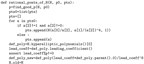
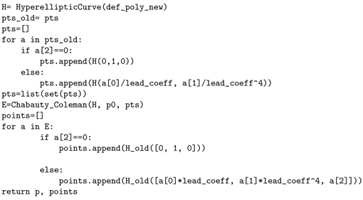
Note that the implementation of this algorithm only took into account the hyperelliptic curves defined by a polynomial monic [5]. Since, in most of the cases that have processed the hyperelliptic curve it was defined by a polynomial no monic. So we had to add to the code in Sage of [6] a function allowing this algorithm to take into account polynomial not necessarily monic.

Here we present the code for this function in SageMath Software [12].

We give below the steps of Algorithm 4, for more details see [5].

Step 1 (Required precision.) We need to choose the p-adic precision N and the t-adic precision M to guarantee that, in Step 3, we will obtain all the roots of $f_i\left(pt\right)$ in ${\mathbb{Z}}_p$. Set $N=2p+4$ and $M=2p+1$ is sufficient for p prime $p>2g=6$ [2].

Algorithm 4. Chabauty-Coleman method for genus 3 rank 0 hypperelliptic curve.

Step 2 (Annihilator) A basis of the space of differentials $H^0\left({C^{\prime }}_{{\mathbb{Q}}_p}\mathrm{,}{\Omega }^1\right)$ ; is given by $\left\{{\omega }_0\mathrm{,}{\omega }_1\mathrm{,}{\omega }_2\right\}$ where ${\omega }_i=\left(x^i/2y\right)dx$. For each $i=\mathrm{0\; <mo>\; ;\; </mo>1\; <mo>\; ;\; </mo>2}$, define:

$f_i\left(z\right)={\displaystyle {\int }_{\infty }^z{\omega }_i}$

where $\infty$ denotes the point at infinity. The functions $f_i\left(z\right)$ are zero on all rational points of $C^{\prime }$, but not identically zero.

Step 3 (Searching in residue discs.) For each point $\bar{P}\in C\left({\mathbb{F}}_p\right)$, we compute the set of ${\mathbb{Q}}_p$ -rational points P reducing to $\bar{P}$ such that $f_i\left(P\right)=0$ for $i=\mathrm{0\; <mo>\; ;\; </mo>1\; <mo>\; ;\; </mo>2}$. To perform this computation, we consider two different cases:

1) If there is a point $P\in C^{\prime }{\left(\mathbb{Q}\right)}_{known}$ reducing to $\bar{P}$, then we expand each ${\omega }_i$ in terms of a uniformizer t at P and we formally integrate to obtain three power series $f_i\left(t\right)$, that parametrize the integrals of the ${\omega }_i$ between P and any other point in the residue disc.

2) Otherwise, we start by finding a $Q_p$ -point P reducing to $\bar{P}=\left({\bar{x}}_0\mathrm{<mo>\; ;\; </mo>}{\bar{y}}_0\right)$ (note that $\bar{P}$ cannot be $\infty$ in this case). If ${\bar{y}}_0=0$ we can take $P=\left({\bar{x}}_0\mathrm{<mo>\; ;\; </mo>0}\right)$ where $x_0$ is the Hensel lift of $\overline{x_0}$ to a root of $F\left(x\right)$. Otherwise, we can take $P=\left(x_0\mathrm{<mo>\; ;\; </mo>}{y}_0\right)$ where $x_0$ is any lift of $x_0$ to ${\mathbb{Z}}_p$ and $y_0$ is obtained from $y_0$ by applying Hensels Lemma to $y^2=F\left(x_0\right)$. Then we set $f_i\left(t\right)={\bar{f}}_i\left(t\right)+{\displaystyle {\int }_{\infty }^z{\omega }_i}$ ; where each ${\bar{f}}_i\left(t\right)$ parametrizes the integral of ${\omega }_i$ between P and any other point in the residue disc.

Step 4 (Identifying the rational points.) Now, for each of the points Q found in Step 3, we attempt to reconstruct Q as a Q-rational point, using Sage. If this is not possible, then $\left[Q-\infty \right]$ must be a torsion point in $J\left({\mathbb{Q}}_p\right)$, because J has rank 0.

Once we have the rational points of $C^{\prime }$ we can reconstruct the rational points of C. Note that C has the same number of rational points as $C^{\prime }$ and being a curve given by a model of even degree, it has two points at infinity that we note ${\infty }^{+}$ and ${\infty }^{-}$.

We use above algorithms to determine the rational points of C from the rational points of $C^{\prime }$ (Algorithm 5).

Note also that, if after reconstruction, we do not have the at inifinity, we must

Algorithm 5. Computation of the rational points of C.

add them because they are known in advance in our case these are the coordinate points $\left(\mathrm{1\; <mo>\; :\; </mo>1\; <mo>\; :\; </mo>0}\right)$ and $\left(\mathrm{1\; <mo>\; :\; </mo>}-\mathrm{1\; <mo>\; :\; </mo>0}\right)$.

5. Example

We run our algorithms in Sage on a list of 47 hyperelliptic curves of genus 3 and rank 0, obtained from the database [7] giving the models of even degree polynomials having at least one root in $\mathbb{Q}$.

Our implementation proves that for each of the studied curves, the set of rational points is equal to the set of rational points of naive height at most 10⁵.

Figure 1 shows how many of the curves in our list have certain number of rational points.

We observe that the maximun of the points is 4 and that a majority of the curves have three rational points.

We conclude this section, showing how the algorithms work on a particular curve and we show an example of a curve which does not have rational points at infinity.

5.1. Example

Consider a hyperelliptic curve C of genus 3 given by:

$C\mathrm{<mo>\; :\; </mo>}{y}^2=x^8-4x^7+4x^6+2x^5-8x^4+8x^3+x^2-4x$.

The function RankBound in Magma shows that the jacobian J of C has a rank of Mordell-Weil 0. Then we can apple the algorithms described above to compute the number of rational points of C. We proceed as follows:

Let’s pose $f\left(x\right)=x^8-4x^7+4x^6+2x^5-8x^4+8x^3+x^2-4x$. It is easy see that f vanishes into $0\in \mathbb{Q}$. Therefore, the curve C is $\mathbb{Q}$ -isomorphic a imaginary hyperelliptic curve that denote $C^{\prime }$.

Step 1: Compute of the equation of C'

Let $y^2=F\left(x\right)$ the equation of the curve $C^{\prime }$. By Algorithm 3, we have $F\left(x\right)=x^{8}f\left(\frac{1+ax}{x}\right)$ with $a=0$, then $C^{\prime }$ is given by:

$C^{\prime }\mathrm{<mo>\; :\; </mo>}{y}^2=-4x^7+x^6+8x^5-8x^4+2x^3+4x^2-4x+1$.

Figure 1. Number of hyperelliptic curves of genus 3 given by a model of even degree in the list and n points rationels.

Step 2 Computing rational points of C'

Using Magma we find that the set of rational points of $C^{\prime }$ with a height bounded by 10⁵ is:

$C^{\prime }{\left(\mathbb{Q}\right)}_{\text{know}}=\left\{\infty \mathrm{,}\left(\mathrm{0,}-1\right)\mathrm{,}\left(\mathrm{0,1}\right)\mathrm{,}\left(\mathrm{1,0}\right)\right\}$.

Since the curve has good reduction modulo 7 > 6, we run the Algorithm 4 using this prime. The points of $C^{\prime }\left({\mathbb{F}}_7\right)$ are as follows:

$\left\{\bar{\infty }\mathrm{,}\overline{\left(\mathrm{1\; <mo>\; ;\; </mo>0}\right)}\mathrm{,}\overline{\left(\mathrm{0\; <mo>\; ;\; </mo>1}\right)}\mathrm{,}\overline{\left(\mathrm{0\; <mo>\; ;\; </mo>6}\right)}\right\}$.

After Hensel lifting each of these points to a point of $C^{\prime }\left({\mathbb{Q}}_7\right)$, we write $f_0\left(z\right)\mathrm{,}{f}_1\left(z\right)$ and $f_2\left(z\right)$ in local coordinates, we obtained:

$\begin{array}{c}{f}_0\left(z\right)=-\frac{1}{4}z-\frac{9}{32}{z}^3-\frac{1767}{2560}{z}^5-\frac{62103}{28672}{z}^7-\frac{9063575}{1179648}{z}^9\\ -\frac{338395653}{11534336}{z}^{11}-\frac{25665563035}{218103808}{z}^{13}+O(\; z\; 15\; )\end{array}$

$\begin{array}{c}{f}_1\left(z\right)=-\frac{1}{4}z-\frac{25}{96}{z}^3-\frac{321}{512}{z}^5-\frac{55933}{28672}{z}^7-\frac{8124485}{1179648}{z}^9\\ -\frac{302419335}{11534336}{z}^{11}-\frac{22889075713}{218103808}{z}^{13}+O(\; z\; 15\; )\end{array}$

$\begin{array}{c}{f}_2\left(z\right)=-\frac{1}{4}z-\frac{23}{96}{z}^3-\frac{1451}{2560}{z}^5-\frac{50195}{28672}{z}^7-\frac{7261675}{1179648}{z}^9\\ -\frac{269617641}{11534336}{z}^{11}-\frac{20370900655}{218103808}{z}^{13}+O\left(z^{15}\right)\end{array}$.

Then we use the PARI/GP function polrootspadic to compute the common zeros of the $f_0\left(z\right)\mathrm{mod}{7}^{18}$, $f_1\left(z\right)\mathrm{mod}{7}^{18}$ and $f_2\left(z\right)\mathrm{mod}{7}^{18}$. We notice, that they have the common zeros in the discs $\bar{\infty }\mathrm{,}\overline{\left(\mathrm{1\; <mo>\; ;\; </mo>0}\right)}\mathrm{,}\overline{\left(\mathrm{0\; <mo>\; ;\; </mo>1}\right)}$ and $\overline{\left(\mathrm{0\; <mo>\; ;\; </mo>6}\right)}$ which correspond respectively to the points $\infty \mathrm{,}\left(\mathrm{1,0}\right)\mathrm{,}\left(\mathrm{0,1}\right)$ and $\left(\mathrm{0,}-1\right)$.

Therefore, we have shown that $C^{\prime }\left(\mathbb{Q}\right)=\left\{\infty \mathrm{,}\left(\mathrm{0\; <mo>\; ;\; </mo>}-1\right)\mathrm{,}\left(\mathrm{0\; <mo>\; ;\; </mo>1}\right)\mathrm{,}\left(\mathrm{1\; <mo>\; ;\; </mo>0}\right)\right\}$.

Step 3 Determination of the rational points of C

We now move on to the phase of constructing the rational points of C from $C^{\prime }\left(\mathbb{Q}\right)$ using Algorithm 5. We start adding the point used for the variable change i.e.: $P1\left(a=\mathrm{0\; <mo>\; ;\; </mo>0}\right)$ and the points at infinity ${\infty }^{+}$ and ${\infty }^{-}$. Let $Q=\left(\mathrm{1,0}\right)\in C^{\prime }\left(\mathbb{Q}\right)$, we compute the point $P2\left(x\mathrm{<mo>\; ;\; </mo>}y\right)\in C\left(\mathbb{Q}\right)$ such that

$x=\frac{1+a{x}^{\prime }}{x^{\prime }}$ and $y=\frac{y^{\prime }}{{x^{\prime }}^4}$ Hence $P2=\left(\mathrm{1\; <mo>\; ;\; </mo>0}\right)$. Since Q is the only point in $C^{\prime }$

whose the x-coordinate is different from $a=0$, Algorithm 5 stops here. Therefore:

$C\left(\mathbb{Q}\right)=\left\{{\infty }^{+}\mathrm{,}{\infty }^{-}\mathrm{,}\left(\mathrm{0\; <mo>\; ;\; </mo>0}\right)\mathrm{,}\left(\mathrm{1\; <mo>\; ;\; </mo>0}\right)\right\}$.

We check that we have the same result using Magma with a height of 10⁵.

In our list, we found case of a hyperelliptic curve whose polynomial f is not monic and its leading coefficient is not a square in $\mathbb{Q}$. So the curve has no pints at infinity. We present it in the following example.

5.2. Example

Let be the hyperelliptic curve:

$C\mathrm{<mo>\; :\; </mo>}{y}^2=-3x^8-8x^7-18x^6-18x^5-15x^4+2x^3+5x^2+8x$.

This curve does not have rational points at infinity since the leading coefficient of the polynomial defining the curve is not a square in $\mathbb{Q}$.

By Algorithm 3, the curve C is transformed into the imaginary hyperelliptic curve $C^{\prime }$ given by:

$C^{\prime }\mathrm{<mo>\; :\; </mo>}{y}^2=8x^7+5x^6+2x^5-15x^4-18x^3-18x^2-8x-3$.

Using Magma, we have:

$C^{\prime }{\left(\mathbb{Q}\right)}_{\text{know}}=\left\{\infty \right\}$.

Since the curve has good reduction modulo 7, we run Algorithm 4 and we find that $C^{\prime }\left(\mathbb{Q}\right)=\left\{\infty \right\}$.

Since $C^{\prime }$ has only one rational point, then C will only have one rational point too which will be none other than the point used for the change of variable. By Algorithm 5, we get $C\left(\mathbb{Q}\right)=\left\{\left(\mathrm{0,0}\right)\right\}$.

6. Conclusion

In this paper, we have presented the computation of rational points on hyperelliptic curves of genus 3 given by an even degree model and whose Jacobian has a Mordell-Weil rank 0, using the isomorphism between the real hyperelliptic curve and the imaginary hyperelliptic curve. Our calculations show that the rational points on C are the same as when we search on Magma with a height of at most 10⁵.

Conflicts of Interest

The authors declare no conflicts of interest regarding the publication of this paper.

References

[1]	Coleman, R.F. (1985) Effective Chabauty. Duke Mathematical Journal, 52, 765-770. https://doi.org/10.1215/S0012-7094-85-05240-8
[2]	Balakrishnan, J.S., Bianchi, F., Cantoral-Farfán, V., Çiperiani, M. and Etropolski, A. (2018) Chabauty-Coleman Experiments for Genus 3 Hyperelliptic Curves. In: Balakrishnan, J., Folsom, A., Lalín, M. and Manes, M., Eds., Research Directions in Number Theory, Springer, Cham, 67-90. https://doi.org/10.1007/978-3-030-19478-9_3
[3]	Balakrishnan, J.S. (2015) Coleman Integration for Even-Degree Models of Hyperelliptic Curves. LMS Journal of Computation and Mathematics, 18, 258-265. https://doi.org/10.1112/S1461157015000029
[4]	Balakrishnan, J.S., Bradshaw, R.W. and Kedlaya, K.S. (2010) Explicit Coleman Integration for Hyperelliptic Curves. In: Hanrot, G., Morain, F. and Thomé, E., Eds., Algorithmic Number Theory, ANTS 2010. Lecture Notes in Computer Science. Springer, Berlin, 16-31. https://doi.org/10.1007/978-3-642-14518-6_6
[5]	de Frutos Fernaandez, M.I. and Hashimoto, S. (2019) Computing Rational Points on Rank 0 Genus 3 Hyperelliptic Curves. arXiv, 190904808v2, 1-10.
[6]	de Frutos Fernaandez, M.I. and Hashimoto, S. (2019) Sage Code. https://github.com/sachihashimoto/rational-points-hyperelliptic
[7]	Booker, A., Platt, D., Sijsling, J. and Sutherland, A. (2018) Genus 3 Hyperelliptic Curves. 1-4. http://math.mit.edu/~drew/lmfdb_genus3_hyperelliptic.txt
[8]	Jacobson, M.J., Scheidler, R. and Stein, A. (2009) Cryptographic Aspects of Real Hyperelliptic Curves. Cryptology ePrint Archive, 1-28.
[9]	Stoll, M. (2014) Arithmetic of Hyperelliptic Curves. Screen Version of August 1, 2014, 1, 1-35.
[10]	McCallum, W. and Poonen, B. (2012) The Method of Chabauty and Coleman, Explicit Methods in Number Theory. In: Panoramas et Synthèses, Société Mathématique de France, Paris, 36, 99-117.
[11]	Balakrishnan, J.S. (2011) Coleman Integration for Hyperelliptic Curves: Algorithms and Applications. Thesis, Massachusetts Institute of Technology, Cambridge, MA, USA.
[12]	Zimmermann, P. (2017) The Sage Developers Sagemath, the Sage Mathematics Software System (Version 9.1).