Six-Element Yagi Array Designs Using Central Force Optimization with Pseudo Random Negative Gravity

Richard A. Formato

Cataldo & Fisher, LLC, Woburn, USA.

DOI: 10.4236/wet.2021.123003                

Abstract

A six-element Yagi-Uda array is optimally designed using Central Force Optimization (CFO) with a small amount of pseudo randomly injected negative gravity. CFO is a simple, deterministic metaheuristic analogizing gravitational kinematics (motion of masses under the influence of gravity). It has been very effective in addressing a wide range of antenna and other problems and normally employs only positive gravity. With positive gravity the six element CFO-designed Yagi array described here exhibits excellent performance with respect to the objectives of impedance bandwidth and forward gain. This paper addresses the question of what happens when a small amount of negative gravity is injected into the CFO algorithm. Does doing so have any effect, beneficial, negative or neutral? In this particular case negative gravity improves CFO’s exploration and creates a region of optimality containing many designs that perform about as well as or better than the array discovered with only positive gravity. Without some negative gravity these array configurations are overlooked. This Yagi-Uda array design example suggests that antennas optimized or designed using deterministic CFO may well benefit by including a small amount of negative gravity, and that the negative gravity approach merits further study.

Keywords

Antenna, 6-Element Array, Yagi, Yagi-Uda, Array, Impedance Bandwidth, VSWR, Forward Gain, Antenna Design, Antenna Optimization, Central Force Optimization, CFO, Deterministic, Metaheuristic, Evolutionary Algorithm, Gravity, Gravitational Kinematics, Exploration, Exploitation

1. Introduction

The Yagi-Uda array (Yagi) has been around for nearly one hundred years [1] [2], undoubtedly because of its ability to provide excellent performance across a wide range of antenna measures, always in a simple geometry and often in a compact one as well [3]. The basic Yagi comprises a single driven dipole element (DE) flanked by a single parallel parasitic reflector (REF) on one side and any number of parasitic parallel directors on the other (D_i). A typical six-element geometry is shown in Figure 1 (red dot marking DE feedpoint). The X-axis is the Yagi’s “boom”, and the array’s elements are an arranged along it in the X-Y plane parallel to each other and to the Y-axis as shown. REF, the element that is closest to the Y-axis, is closer to DE than the first director and longer than DE while the D_i are shorter, but these characteristics do not by any means constitute absolute design requirements, as they simply are typical geometry that produces appropriate phase and current relationships between the array elements.

A complete Yagi design must include the lengths and diameters of each element and the inter-element spacings. A six-element array thus has seventeen design parameters (six element lengths, six diameters, and five spacings). If the feedpoint input impedance is considered a design variable as well (discussed below), then the design/optimization (D/O) problem comprises eighteen dimensions. Many Yagis have far more than six elements, and every additional one adds three more design parameters (variables) to the problem.

There is no accurate analytical approach to Yagi array design using models that assume purely sinusoidal element current distributions and that neglect their mutual couplings. These assumptions lead to inaccuracies, and as a result many design approaches are inherently approximate or based entirely on empirical data [3] [4] [5]. The difficulty in analytically calculating a Yagi’s element currents is highlighted by the fact that there is no known formula for expressing the current distribution on even the simplest of radiating elements, a single center fed dipole in free space [6].

2. Methodology

2.1. Background

Over the past two decades or so, in response to the limitations described above, Yagi D/O largely has been done using metaheuristics, that is, algorithms that provide acceptable solutions in reasonable times without being exact or having a

Figure 1. Schematic 6-Element Yagi.

mathematical proof that the optimal solution eventually will be found [7]. Many Global Search and Optimization (GSO) algorithms have been applied to the Yagi design problem against a variety of performance measures using various techniques, as examples: Gain, impedance, bandwidth using Particle Swarm Optimization (PSO) [8]; Yagi design using Multi-Objective Differential Evolution (DE) [9]; 6-Element array design based on Gain-Impedance Multiobjective Optimization [10]; Overview of Yagi design methods, many of them GSO’s [11]; Evolutionary methods for Yagi design [12]; Maximum gain optimization using Biogeography Based Optimization (BBO) variants [13]; Ultrawideband 6-element Yagi design using CFO/Variable Z₀ [14]; 6-Element Yagi design using Dominating Cone Line Search (DCLS) [15]; Dipole array optimization using Fitness-Adaptive DE [16]; Yagi design using Genetic Algorithms [17]; Wideband 6-element Yagi design using Adaptive DE [18]. These are only a sampling of the dozens if not hundreds of GSO approaches to Yagi-Uda array design.

This paper reports results for a typical 6-element Yagi design developed with a basic Central Force Optimization (CFO) implementation that includes a small amount of pseudo randomly injected negative gravity. CFO is a deterministic evolutionary metaheuristic that analogizes gravitational kinematics (motion of masses under the influence of gravity) [19], and it has been applied to antenna D/O on a variety of structures, [20] - [28] being representative examples. CFO and modifications have been further developed and applied to a variety of other problems as well, [29] - [38] serving as examples. CFO is fundamentally deterministic, which in fact was a prime consideration in its formulation. Every CFO run with the same setup yields the same results, thereby eliminating the need for statistical analysis of possibly hundreds or even thousands of runs as required by fundamentally stochastic GSO’s. Determinism can be very important in dealing with “real world” antenna problems, and also others, because one of the unknowns in a real problem is defining a suitable fitness function. This task is made much simpler by using a metaheuristic whose results depend only on user input and not on the randomness of a stochastic algorithm. This issue is discussed in detail with examples in [39].

CFO explores a D/O problem’s landscape by flying through its decision space (DS) “probes” whose trajectories are governed by equations analogous to those governing gravitational kinematics. DS comprises vectors $X=\left(x_1,\cdots ,x_{N_d}\right)$ whose components x_i are the N_d Yagi array design (decision) variables (element lengths, spacings, diameters, and Z₀) with their allowable ranges (min/max values for each). Each such vector represents a complete array design. A CFO run begins with an Initial Probe Distribution (IPD) whose configuration is determined by the algorithm designer. The possibilities are limitless, and some IPD’s work better than others. In many recent CFO implementations a “probe line” IPD has been used in which CFO’s probes are arranged uniformly on lines parallel to the DS axes and intersecting along DS’s principal diagonal. For the work reported here, however, a pseudo random π-fraction IPD was used because it is simpler. π-fractions also were used to determine the degree of injected negative gravity. As a result, and as expected, the target and actual levels of negative gravity are not precisely equal.

Even though CFO is deterministic, it is reasonable to speculate that CFO may benefit from the inclusion of a pseudo random component. A pseudo random variable (prv) is a number known precisely by enumeration or calculation, in contrast to a true random variable (rv) whose value is a priori unknowable because it must be calculated from a probability distribution. With respect to any D/O problem, the prv is “random” in the sense that it is uncorrelated with the problem’s topology (“landscape”). Additionally, the prv’s themselves must be uniformly distributed and uncorrelated. Pseudo randomness is included here using π-fractions generated by the Bailey-Borwein-Plouffe (BBP) algorithm. A detailed discussion of π-fractions and their use in a sample GSO algorithm, πGASR (Genetic Algorithm with Sibling Rivalry), appears in [40].

2.2. CFO Run Setup

A detailed description of the basic CFO algorithm is in the Appendix Part 2. Run parameters and the decision space boundaries for the basic CFO implementation used in this paper appear in Table 1 and Table 2 and are discussed in detail in the Appendix. For this particular problem the Yagi element radius was fixed at 0.00635 m (1/2 inch diameter to facilitate easier fabrication). This simplification results in eleven geometric variables instead of seventeen. The twelfth variable to be determined by CFO is Z₀, the Yagi’s feedpoint impedance. Variable Z₀ (VZ₀) is a patented “product-by-process” technology in which the antenna’s feedpoint impedance is treated as an optimization variable rather than as a fixed parameter as usually is the case. At this time VZ₀ is publicly available for use by anyone who wishes to use it (U.S. Patent No. 8,776,002). CFO pseudo code appears in Figure 2, and the source code used to generate the data presented here is available on request to the author ([e-mail]).

Table 1. CFO run parameters.

Table 2. Decision space boundaries.

Figure 2. CFO pseudo code [41].

2.3. Exploration vs. Exploitation in CFO

Positive gravity causes CFO’s probes always to move toward greater fitnesses, never away, and consequently to some degree perhaps to impede CFO’s exploration. CFO often converges very quickly [42], which is a favorable attribute, but not if it is at the expense of under-sampling DS, which may be the case. This paper speculates that adding some negative gravity causing probes to fly away from each other may improve CFO’s exploration because probes that otherwise would coalesce will explore further by flying into DS regions that have been under-sampled or perhaps not sampled at all. The effect of negative gravity is well illustrated in the discussion and figures in Section 6 of [43], and parameter values that insure CFO’s convergence on maxima are discussed in [44].

With respect to G’s sign, + or ‒, the specific question is, Does making it negative benefit CFO’s performance, and if so, why? Or does it impede it, and if so, why? To quote:

“‘Exploration and exploitation are the two cornerstones of problem solving by search.’ For more than a decade, Eiben and Schippers’ advocacy for balancing between these twoantagonistic cornerstones still greatly influences the research directions of evolutionary algorithms (EAs)...” [45], emphasis added. This issue also is discussed in [46] [47] [48]. Like all GSO algorithms CFO is subject to the inescapable tension between exploration (adequately sampling DS) and exploitation (quickly converging on global maxima). The test case reported here shows that a small amount of negative gravity indeed does benefit CFO’s performance, ostensibly because it enhances CFO’s exploration while retaining the algorithm’s ability to exploit already located maxima.

At each step negative gravity was pseudo randomly injected into CFO using π-fractions whose values are input from an external file containing the BBP-computed fractions π_k, 1 ≤ k ≤ 215829 (k is the π-fraction index). In order to avoid correlations between the π-fractions (see [40] ), k is incremented by 5 at each step. If k exceeds 215829 it is reset to max(k-215827,3). The parameter 0 ≤ P_neg ≤ 100 specifies the target amount of negative gravity in percent, for example, P_neg = 6.5 sets the target at 6.5%. At each step the then current value of π_k is tested against P_neg to determine whether or not gravity is negative at that step. Specifically, if π_k ≤ P_neg/100 then $G=-\left|G\right|$ (negative gravity), otherwise $G=\left|G\right|$ (positive gravity). Because prv’s are used, the nature of gravity at each step is a priori known precisely and is uncorrelated with the outcome at any other step. Also because prv’s are used, the desired (target) level of negative gravity and the actual level will not be precisely equal. As the CFO run includes more and more steps the difference between actual and target levels of G ≤ 0 grows smaller with a limiting value of zero because the π-fraction prv’s are uniformly distributed. For this Yagi D/O problem runs were made with non-uniformly spaced values of P_neg in [0, 20%]. The actual vs. target levels of G ≤ 0 is plotted in Figure 3 and shows good agreement.

Every CFO run comprised 550 steps, a large enough number to meet several

Figure 3. Actual vs Target Neg. Gravity with 550 Steps.

objectives: 1) allow fitness evolution essentially to saturate (more steps resulting only in incremental improvement); 2) create actual an actual degree of G ≤ 0 close to the target value; and 3) reasonable runtimes (~8 min on Win7/HP 64-bit SP1; Intel Core i7 4700MQ 2.4 GHZ). Because there is no accurate analytical model of the six-element Yagi-Uda array, the performance of each candidate design evolved by CFO was modeled using the NEC-4 Method of Moments code [49] whose accuracy is well established. Another version of NEC was used in the program 4nec2 (below) to compute and visualize performance data for the two CFO-optimized arrays at 0% and 6% G < 0 over a very wide frequency range (data in Appendix Part 1).

2.4. Fitness Function

The performance of every candidate antenna design was measured by the following simple fitness function (of course, the choice of fitness function is entirely up to the algorithm designer):

$F=c_1\cdot g_{\text{L}}+c_3\cdot g_{\text{M}}+c_5\cdot g_{\text{U}}-c_2\cdot S_{\text{L}}-c_4\cdot S_{\text{M}}-c_6\cdot S_{\text{U}}$ (1)

where subscripts L, M, and U denote lower, mid and upper frequencies at which the Yagi’s power gain, g, and feedpoint voltage standing wave ratio, S (not to be confused with spacing), are computed. The weights $c_1=c_2=c_5=c_6=1$ and $c_{\text{3}}=c_{\text{4}}=\text{3}$ were chosen for simplicity while intentionally favoring midband performance, slightly, with L = 294.8 MHz, M = 299.8 MHz, U = 304.8 MHz. VSWR (Voltage Standing Wave Ratio) is computed relative to the feed point impedance Z₀ and denoted VSWR//Z₀. While Z₀ usually is a fixed, user-supplied parameter, typically the industry standard value of 50 Ω, VZ₀ treats it the same as any other decision space variable. This approach embraces array current distributions that otherwise would be excluded because they fail to adequately match a predetermined value of Z₀. Whether or not the CFO-returned value is feasible and desirable is an engineering and economic judgment, and more often than not it is worth impedance-matching the “non-standard” Z₀because the antenna’s performance is better, often much better [50]. At each of the three frequencies L, M, U, NEC-4 returned the Yagi’s maximum gain and feedpoint impedance. Appendix Part 1 contains additional performance data computed with the freely available program 4nec2 that facilitates visualization of its computed data [51].

3. Results

3.1. Fitness Evolution

The reference Yagi design for this study is, of course, the one that CFO generates with zero negative gravity, the usual CFO implementation. Figure 4(a) and Figure 4(b) plot CFO’s fitness evolution as a function of Step Number with zero and 6 percent negative gravity, respectively. The maximum fitnesses are 47.8932 (0% G < 0) and 49.1892 (6% G < 0). Not only does injecting a small amount of negative gravity result in a slightly better fitness, but the fitness evolves quite differently with the 6% curve rising far more quickly than the 0% curve and with saturation taking place faster. This CFO implementation does not employ elitism (always including the best global fitness), so that here the best fitness at each step is a function only of the then current probe distribution.

How the fitness varies with the amount of negative gravity is plotted in Figure 5. For values below about 6% the fitness drops appreciably from its 0% value, but then it quickly recovers reaching a value higher than at 0% G ≤ 0 and settling into a plateau-like region up to about 10% G ≤ 0. Thereafter the fitness decreases monotonically through the test range of about 20%. The fitness plateau between approximately 6% and 10% is marked the “~region of optimality” on the plot because in that range the fitness is more or less flat. Fitness varies from the maximum value of 49.1892 at 6% G < 0 to a minimum of 47.392 at 6.36% G < 0. All other values are in this range, and consequently very similar one to the next and also to the 0% G < 0 value.

Figure 4. (a). Fitness Evolution with Zero Neg. Gravity; (b) Fitness Evolution with 6% Neg. Gravity.

Figure 5. Fitness vs amount of injected negative gravity.

Returning to the fundamental question addressed in this paper, Has pseudo randomly adding a small amount of negative gravity improved CFO’s exploration of the six-element Yagi’s decision space? The fitness data clearly show that the answer is “yes.” However, adding too much G < 0 prevents CFO from exploiting the solutions it has found. How much negative gravity is appropriate no doubt is problem-specific, but this array design example strongly suggests that every CFO implementation should experiment with some measure of G < 0.

3.2. Average Probe Distance

Step-by-step the normalized average distance from the probe with the best fitness to all other probes, denoted D_avg, is a good measure of CFO’s convergence (see Appendix Part 2 for details). In many cases it approaches zero meaning that all probes have very tightly coalesced around the probe with the best fitness (maximum value). In other cases, such as here, the probe distribution more or less stabilizes but on average at some distance from the best probe.

Figure 6 plots D_avg for the cases of zero negative gravity, (a), and for 6% G < 0, (b). Both cases initially show an extreme oscillation that diminishes with increasing Step #. This oscillatory behavior in CFO’s D_avg appears to be correlated with local trapping and is not entirely unexpected in view of CFO’s metaphor of gravitational kinematics. In fact, in the real Universe similar oscillatory behavior is seen in the trajectories of Near Earth Objects (NEO’s) that become gravitationally trapped by the Earth’s gravity and eventually break loose without any energy loss [52] [53] [54].

In order to investigate D_avg’s behavior in very long runs, two were made, both with N_t = 10,000 steps, zero negative gravity and at a target value of G < 0 of 5%. As discussed in Section 2.3 the actual and target levels of negative gravity are not equal except in the limit of an infinite number of steps. While both the 550-step

Figure 6. (a) Average distance to best probe, zero neg. gravity; (b) Average distance to best probe, 6% neg. gravity.

and 10,000-step runs targeted G < 0 at 5%, in the first case the actual value was 6% and in the second a much closer 5.22%. The D_avg results, which are quite interesting, are plotted in Figure 7. In both cases, zero and 5.22% G < 0, D_avg settles down to what appears to be a stable, uniform magnitude oscillation with much smaller amplitude in the 5.22% case. In fact, at 5.22% G < 0 D_avg does not oscillate at all, and from steps #676-10,000 it is equal to 0.2352928. CFO’s probe distribution is stable and no longer changes step-to-step. In contrast, for the zero gravity case D_avg oscillates in an erratic but repetitive pattern as seen in the expanded plot for steps 9900 - 10,000, Figure 8. It is reasonable to expect that these behaviors for cases zero and 5.22% G < 0 will continue indefinitely with an increasing number of steps. It is evident from these data that pseudo randomly injecting a small measure of negative gravity indeed does improve CFO’s exploration and apparently eliminates the probe trapping seen in Figure 8 as well.

3.3. Maximum Yagi Gain

The variation of maximum Yagi gain with degree of negative gravity is plotted in Figure 9. The antenna’s maximum gain occurs along the direction of its boom (the +X-axis) at NEC angles θ = 90˚, φ = 0˚ in its right-handed spherical coordinate system (see [49] ). With zero negative gravity the gain is 11.37 dBi, but at 6% G < 0 it increases to 11.92 dBi, which is a significant improvement. The max gain curve mirrors the Figure 8 structure of the fitness curve in Figure 5. Their shapes are very similar, and the array’s maximum gain is highly correlated with the array’s fitness as measured by Equation (1). Figure 10 plots the relative frequency of maximum gain as the percentage deviation from the midband reference frequency of 299.8 MHz. Its shape is quite irregular showing no correlation with either the fitness or maximum gain curves. The frequency of maximum gain is close to 299.8 MHz only for actual G < 0 of ~1.3% and in two narrow bands near 6% and ~11.2%. Otherwise the deviations from midband show considerable variability, ranging as high as nearly +3% and as low as about −2.4%.

Figure 7. (a) Average Distance to Best Probe, Zero Neg. Gravity; (b) Average Distance to Best Probe, 5.22% Neg. Gravity.

Figure 8. Probe average distance oscillation, steps 9900-10000.

Figure 9. Max gain vs injected negative gravity.

Figure 10. Max gain frequency relative to band center.

The array’s relative gain bandwidth

~ region of

optimality

3.4. Voltage Standing Wave Ratio (VSWR)

~ region of

optimality

Figure 11. −3 dB Gain bandwidth relative to band center.

Figure 12 shows the 2:1 VSWR bandwidth in MHz. In the approximate region of optimality it ranges from about 14.5 MHz to just over 20 MHz with much higher values on either side. The tradeoff for increasing impedance bandwidth is maximum gain. The overall best performing arrays discovered by CFO lie in the region of optimality. Figure 13 shows the 2:1 VSWR as a percentage of the midband reference frequency of 299.8 MHz. In the region of optimality it ranges from about 5% to just under 7%, so it is not particularly sensitive to the level of injected negative gravity. Outside this region it does reach higher values, but, again, the tradeoff is with maximum array gain.

Figure 12. 2:1 VSWR bandwidth vs neg. gravity.

Figure 13. 2:1 VSWR fractional bandwidth.

Figure 14. 3:1 VSWR Fractional Bandwidth.

As a final measure of the optimized antennas’ performance Figure 14 plots the fractional 3:1 VSWR BW as a function of percentage G < 0. As expected, the 3:1 impedance bandwidth is much greater than its 2:1 counterpart, quite large in fact over much of the region of optimality But as a practical matter not many communication systems tolerate VSWR’s in the 3:1 range well, and it is a level generally to be avoided if at all possible.

4. Conclusion

This paper reports the results of the D/O of a six-element Yagi-Uda array using Central Force Optimization with pseudo randomly injected negative gravity. Adding 6% G < 0 results in an array that out performs its 0% G < 0 counterpart and also discovers a range of designs with similar fitnesses. Negative gravity was inserted using π-fraction pseudo random variables thereby preserving CFO’s determinism, which is an important consideration in real-world problems that require the formulation of a suitable fitness function. G < 0 has the effect of spreading apart CFO’s probes because negative gravity is repulsive in nature instead of attractive. This wider dispersal improves CFO’s exploration of the decision space without sacrificing the algorithm’s demonstrated high level of exploitation. Injecting some level of negative gravity likely will improve CFO’s exploration across the board, not only in the Yagi array D/O problem but in other applications as well. This particular problem is only one example of the benefit provided by injecting some small measure of negative gravity, and it does not (necessarily) provide specific guidance as to how much G < 0 should be used in any other particular case. The effect of negative gravity in CFO is a research area that should be pursued because the work reported here strongly suggests that there may be considerable benefit in doing so.

Appendix Part 1: Additional Yagi Performance Data

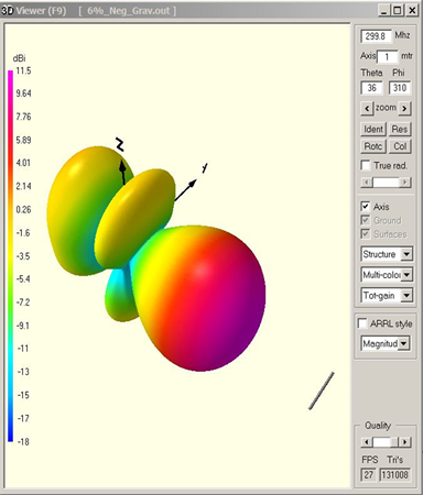
CFO’s best fitness NEC input files at zero and 6% G < 0 fully define the array geometry and Z₀. NEC input files appear immediately below, 0% G < 0 first, followed by 6% G < 0. Dimensions are in meters, and since the wavelength, λ, at 299.8 MHz is 1 m the array dimensions also are in λ. The array can be scaled to any other frequency by scaling its dimensions by the wavelength ratio. Also in this Appendix are screenshots of the 4nec2 (ver. 5.8.17) output: 1) 3D radiation patterns @ 299.8 MHz; 2) power gain, VSWR//Z₀, and feedpoint impedance for 250 - 350 MHz and for 294.8 - 304.8 MHz, and 3) NEC Average Gain Test at 299.8/250/350 MHz.

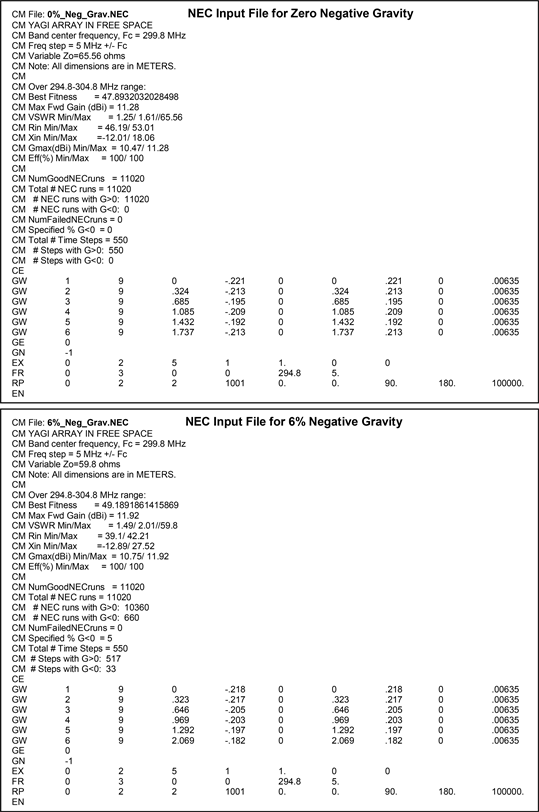
In the following screenshots 0% G < 0 is on the left, 6% G < 0 on the right.

3D Radiation Patterns (299.8 MHz)

4nec2 Summary Data, 299.8 MHz (with Average Gain Test, AGT, results)

Total Gain (dBi), 294.8 - 304.8 MHz (note: 4nec2 does not compute F/B if Gain is selected)

VSWR//Z₀, 294.8 - 304.8 MHz (Z₀ = 65.56Ω @ 0% G < 0; 59.8Ω @ 6% G < 0)

Feedpoint Impedance, 294.8 - 304.8 MHz

Total Gain (dBi), 250 - 350 MHz (note: 4nec2 does not compute F/B if Gain is selected)

VSWR//Z₀, 250 - 350 MHz (Z₀ = 65.56Ω @ 0% G < 0; 59.8Ω @ 6% G < 0)

Feedpoint Impedance, 250 - 350 MHz

4nec2 Summary Data, 0% G < 0, 250 & 350 MHz (including AGT results)

4nec2 Summary Data, 6% G < 0, 250 & 350 MHz (including AGT results)

Appendix Part 2: Basic Central Force Optimization

A2.1. The CFO Metaphor

Central Force Optimization (CFO) analogizes gravitational kinematics, the motions of real bodies in the real Universe under the influence of gravity. The fundamental law of physics is Newton’s Universal Law of Gravitation, according to which the magnitude of the force between the two masses $m_1$ and $m_2$ is given by [55]

$F=\gamma \frac{m_1{m}_2}{r^2}$ (A1)

where r is the distance between them and $\gamma$ the “gravitational constant.” This force always is attractive, never repulsive, and mass in the real Universe always is positive, never negative. The force of gravity is a central force because it acts only along the line connecting the mass centers. Mass $m_1$ experiences a vector acceleration due to mass $m_2$ that is given by

${\stackrel{\to }{a}}_1=-\gamma \frac{m_2\hat{r}}{r^2}$ (A2)

where $\hat{r}$ is a unit vector that points toward $m_1$ along the line joining the masses.

A2.2. Problem Statement

The CFO metaheuristic solves the following problem: In a decision space (DS) defined by $x_i^{\min }\le x_i\le x_i^{\max },i=1,\cdots ,N_d$ where the $x_i$ are decision variables, locate the global maxima of an objective function $f\left(x_1,x_2,\cdots ,x_{N_d}\right)$ possibly subject to a set of constraints $\Omega$ among the decision variables. The value of $f\left(x_1,x_2,\cdots ,x_{N_d}\right)$ is called the “fitness.” CFO explores DS by flying metaphorical “probes” whose trajectories are governed by equations of motion drawn from gravitational kinematics.

A2.3. Constant Acceleration

The vector location of a mass under constant acceleration is given by the position vector [56]

$\stackrel{\to }{R}\left(t+\Delta t\right)={\stackrel{\to }{R}}_0+{\stackrel{\to }{V}}_0\Delta t+\frac{1}{2}\stackrel{\to }{a}\Delta t^2$ (A3)

where $\stackrel{\to }{R}\left(t+\Delta t\right)$ is the position at time $t+\Delta t$. ${\stackrel{\to }{R}}_0$ and ${\stackrel{\to }{V}}_0$, respectively, are the position and velocity vectors at time t, and the acceleration $\stackrel{\to }{a}$ is constant during the interval $\Delta t$. In standard three dimensional Cartesian coordinates $\stackrel{\to }{R}=x\hat{i}+y\hat{j}+z\hat{k}$, where $\hat{i},\hat{j},\hat{k}$ are the unit vectors along the $x,y,z$ axes, respectively. The CFO metaphor analogizes Equations (A1)-(A3) by generalizing them to a decision space of $N_d$ dimensions.

A2.4. Probe Trajectory

CFO’s probes in a typical three-dimensional DS are shown schematically in FigureA1. The location of each probe at each time step is specified by its position vector ${\stackrel{\to }{R}}_j^p$, in which p and j are the probe number and time step index, respectively.

In an $N_d$ -dimensional DS the position vector is ${\stackrel{\to }{R}}_j^p={\displaystyle \underset{k=1}{\overset{N_d}{\sum }}{x}_k^{p,j}}{\hat{e}}_k$, where the $x_k^{p,j}$ are probe p’s coordinates at time step j, and following standard notation ${\hat{e}}_k$ is the unit vector along the $x_k$ axis.

Consider a typical probe,p. It moves from position ${\stackrel{\to }{R}}_{j-1}^p$ at time step $j-1$ to position ${\stackrel{\to }{R}}_j^p$ at time step j under the influence of the metaphorical “gravitational” forces that act on it. Those forces are created by the fitness at each of the other probes’ locations at time step $j-1$. The “time” interval between steps $j-1$ and j is $\Delta t$.

At time step $j-1$ at probe p’s location the fitness is $M_{j-1}^p=f\left(x_1^{p,j-1},x_2^{p,j-1},\cdots ,x_{N_d}^{p,j-1}\right)$. Each of the other probes also has associated with it a fitness of $M_{j-1}^k,k=1,\cdots ,p-1,p+1,\cdots ,N_p$, $N_p$ being the total number of probes. In this illustration, the value of the fitness is represented by the size of the blackened circle at the tip of the position vector. In keeping with the gravity metaphor, the blackened circles may be thought of as “planets,” say, in our Solar System. Larger circles correspond to greater fitness values, that is, bigger planets with correspondingly greater gravitational attraction. In FigureA1 the fitnesses ordered from greatest to least occur at ${\stackrel{\to }{R}}_{j-1}^s$, ${\stackrel{\to }{R}}_j^p$, ${\stackrel{\to }{R}}_{j-1}^n$, and ${\stackrel{\to }{R}}_{j-1}^p$, respectively, as shown by the relative size of the circles.

Probe p’s trajectory in moving from location ${\stackrel{\to }{R}}_{j-1}^p$ to ${\stackrel{\to }{R}}_j^p$ is determined by its initial position and by the total acceleration produced by the “masses” that are created by the fitnesses (or some function defined on them) at each of the other probes’ locations. In the CFO implementation used in this paper the “acceleration,” analogous to Equation (A2), experienced by probe p due to the single probe n is given by

Figure A1. Typical 3-D CFO decision space.

$\frac{G\cdot U\left(M_{j-1}^n-M_{j-1}^p\right)\cdot {\left(M_{j-1}^n-M_{j-1}^p\right)}^{\alpha }\cdot \left({\stackrel{\to }{R}}_{j-1}^n-{\stackrel{\to }{R}}_{j-1}^p\right)}{{\left|{\stackrel{\to }{R}}_{j-1}^n-{\stackrel{\to }{R}}_{j-1}^p\right|}^{\beta }}$ (A4)

where G is CFO’s “gravitational constant” corresponding to $\gamma$ in Equation (A1). Note that in the real Universe $G>0$, always. In CFO space, however, G can be positive (attractive force of gravity) or negative (repulsive force of gravity). Returning to the forces acting on probe p, in a similar fashion to probe n’s effect, the acceleration of probe p due to a different probe s is given by

$\frac{G\cdot U\left(M_{j-1}^s-M_{j-1}^p\right)\cdot {\left(M_{j-1}^s-M_{j-1}^p\right)}^{\alpha }\cdot \left({\stackrel{\to }{R}}_{j-1}^s-{\stackrel{\to }{R}}_{j-1}^p\right)}{{\left|{\stackrel{\to }{R}}_{j-1}^s-{\stackrel{\to }{R}}_{j-1}^p\right|}^{\beta }}$ (A5)

Note that the minus sign in Equation (A2) has been included in the order in which the differences are taken in these acceleration expressions. “Mass” in Equation (A2) corresponds to the terms in the numerator involving the fitnesses. Importantly, it does not correspond to the fitness itself. In these equations $U(\; \cdot \; )$

is the unit step function $U\left(z\right)=\{\begin{array}{l}1,z\ge 0\\ 0,\text{otherwise}\end{array}$. And following standard notation the vertical bars denote vector magnitude, $\left|\stackrel{\to }{X}\right|={\left({\displaystyle \underset{i=1}{\overset{N_d}{\sum }}{x}_i^2}\right)}^{\frac{1}{2}}$, where $x_i$ are the scalar components of $\stackrel{\to }{X}$.

There are no parameters in Equation (A2) corresponding to the “CFO exponents” $\alpha >0$ and $\beta >0$, nor to the unit step $U(\cdot )$. In real physical space $\alpha$ and $\beta$ would take on values of 1 and 3, respectively. Note, too, that the numerators in Equations (A4) and (A5) do not contain a unit vector like Equation (A2). The exponents are included to give the algorithm designer a measure of flexibility by assigning, if desired, a different variation of gravitational acceleration with mass and with distance.

A2.5. Mass in CFO Space

Two other important differences between real gravity and CFO’s version are: 1) the definition of “mass,” which above is the difference of fitnesses, for example, $M_{j-1}^s-M_{j-1}^p$, not the fitness value itself; and 2) inclusion of the unit step

$U\left(z\right)=\{\begin{array}{l}1,z\ge 0\\ 0,\text{otherwise}\end{array}$. The difference of fitnesses is used to avoid excessive

gravitational “pull” by other close by probes that presumably will have fitnesses with similar values. The unit step is included to avoid the possibility of “negative” mass. In the physical Universe, mass is positive, always, but in CFO-space the mass could be positive or negative depending on which fitness is greater. The unit step forces CFO to allow only positive masses, that is, attractive masses. If negative fitness differences were allowed, then some accelerations would be repulsive instead of attractive, thus forcing probes away from large fitness values instead of towards them. The algorithm designer is free to consider other definitions of mass as well. One possibility, for example, might be a ratio of fitnesses similar to the “reduced mass” concept in gravitational kinematics.

A2.6. Total Acceleration and Position Vector for a Single Probe

Taking into account the accelerations produced by each of the other probes on probe p, the total acceleration experienced by p as it “flies” from position ${\stackrel{\to }{R}}_{j-1}^p$ to ${\stackrel{\to }{R}}_j^p$ is given by the sum of the gravitational effects over all other probes, that is,

${\stackrel{\to }{a}}_{j-1}^p=G{\displaystyle \underset{\begin{array}{c}k=1\\ k\ne p\end{array}}{\overset{N_p}{\sum }}U\left(M_{j-1}^k-M_{j-1}^p\right)\cdot {\left(M_{j-1}^k-M_{j-1}^p\right)}^{\alpha }}\times \frac{\left({\stackrel{\to }{R}}_{j-1}^k-{\stackrel{\to }{R}}_{j-1}^p\right)}{{\left|{\stackrel{\to }{R}}_{j-1}^k-{\stackrel{\to }{R}}_{j-1}^p\right|}^{\beta }}$ (A6)

Probe p’s new position vector at time step j is therefore given by

${\stackrel{\to }{R}}_j^p={\stackrel{\to }{R}}_{j-1}^p+{\stackrel{\to }{V}}_{j-1}^p+\frac{1}{2}{\stackrel{\to }{a}}_{j-1}^p\Delta t^2,j\ge 1$ (A7)

which is the analog to Equation (A3), ${\stackrel{\to }{V}}_{j-1}^p$ being the probe’s “velocity” at the end of time step $j-1$. In Equation (A7) the coefficient 1/2, the velocity term, and the time increment $\Delta t$ have been retained primarily as a formalism to highlight the analogy to gravitational kinematics, but they are not required. For the CFO implementation used here, as a matter of convenience, ${\stackrel{\to }{V}}_{j-1}^p$ and $\Delta t$ were arbitrarily set to zero and unity, respectively. Of course, if desired, a constant value of $\Delta t$ and the factor 1/2 can be absorbed into the gravitational constant G.

A2.7. Errant Probes

An important concern is how to handle an “errant” probe, that is, one that flies outside DS, because it is possible that the total acceleration experienced by a probe will fly it into regions of unfeasible solutions that are beyond the DS boundaries. There are many ways to deal with this contingency, and a simple one was implemented in the basic version of CFO used here, the use of a “repositioning factor,” $0\le F_{rep}\le 1$. This factor is used to reposition an errant probe according to the formulas

$\text{If}{x}_i^{p,j}<x_i^{\min }\therefore x_i^{p,j}=x_i^{\min }+F_{rep}\cdot \left(x_i^{p,j-1}-x_i^{\min }\right)$ (A8)

$\text{If}{x}_i^{p,j}>x_i^{\max }\therefore x_i^{p,j}=x_i^{\max }-F_{rep}\cdot \left(x_i^{\max }-x_i^{p,j-1}\right)$ (A9)

$F_{rep}$ is assigned an initial value and incremented at each step by a fixed amount $\Delta F_{rep}$, and if it exceeds unity is reset to the initial value. This simple approach guarantees that all probes will remain inside the decision space. Note that this procedure is pseudo random in nature, but numerical experiments have shown that it is not as effective as pseudo randomly injecting a small amount of negative gravity.

A2.8. D_avg Convergence Metric

Perhaps the best measure of CFO’s convergence is the “Average Distance”

metric computed as $D_{avg}=\frac{1}{L_{diag}\cdot \left(N_p-1\right)}{\displaystyle \underset{p=1}{\overset{N_p}{\sum }}\sqrt{{\displaystyle \underset{i=1}{\overset{N_d}{\sum }}{\left(x_i^{p,j}-x_i^{p^{*},j}\right)}^2}}}$, where $p^{*}$ is the number of the probe with the best fitness; the superscripts p and j denote, respectively, the probe and step numbers as above; and $L_{diag}=\sqrt{{\displaystyle \underset{i=1}{\overset{N_d}{\sum }}{\left(x_i^{\max }-x_i^{\min }\right)}^2}}$

is the length of the decision space principal diagonal. If every one of CFO’s probes has coalesced onto a single point, then $D_{avg}=0$. How closely this metric approaches zero is a good indicator of how CFO’s probe distribution has evolved around a maxima. $D_{avg}$ also is useful in identifying potential local trapping because oscillatory behavior in a $D_{avg}$ plot appears to signal trapping at a local maxima.

Conflicts of Interest

The authors declare no conflicts of interest.

References

[1]	Uda, S. (1926) On the Wireless Beam of Short Electric Waves. Journal of the Institute of Electrical Engineers (Japan), 46, 273-282.
[2]	Yagi, H. (1928) Beam Transmission of Ultra Short Waves. Proceedings of the IEEE, 85, 1864-1874. https://doi.org/10.1109/JPROC.1997.649674
[3]	Stutzman, W.L. and Thiele, G.A. (2013) Antenna Theory and Design. 3rd Edition, John Wiley & Sons, Inc., Hoboken, Sect. 6.3, 166.
[4]	Ramo, S., Whinnery, J.R. and Van Duzer, T. (1994) Fields and Waves in Communication Electronics. Third Edition, Wiley & Sons, Inc., Hoboken, Sect. 12.22, Yagi-Uda Arrays, 64.
[5]	Viezbicke, P. (1976) Yagi Antenna Design. U.S. Government Printing Office, Washington DC. https://doi.org/10.6028/NBS.TN.688 https://play.google.com/store/books/details?id=mqy0Ta4MglAC
[6]	Balanis, C.A. (2005) Antenna Theory Analysis and Design. 3rd Edition, Wiley-Inter- science, Hoboken, Sect. 9.4.2, 509.
[7]	Glover, F. and Sorensen, K. (2015) Metaheuristics. Scholarpedia, 10, Article No. 6532. https://doi.org/10.4249/scholarpedia.6532
[8]	Rattan, M., Patterh, M.S. and Sohi, B.S. (2008) Optimization of Gain, Impedance, and Bandwidth of Yagi-Uda Array Using Particle Swarm Optimization. International Journal of Antennas and Propagation, 2008, Article ID: 193242. https://doi.org/10.1155/2008/193242
[9]	Goudos, S.K., Siakavara, K., Vafiadis, E.E. and Sahalos, J.N. (2010) Pareto Optimal Yagi-Uda Antenna Design Using Multi-Objective Differential Evolution. Progress in Electromagnetics Research, 105, 231-251. https://doi.org/10.2528/PIER10052302
[10]	Singh, S. and Mittal, E. (2013) Designing Yagi-Uda Antenna Using Gain-Impedance Multiobjective Optimization. Journal of Network and Innovative Computing, 1, 203-213.
[11]	Suna, Y., Zhanga, H., Wen, G. and Wanga, P. (2012) Research Progress in Yagi Antennas. Procedia Engineering, 29, 2116-2121. https://doi.org/10.1016/j.proeng.2012.01.272
[12]	Lohn, J.D., Kraus, W.F. and Colombano, S.P. (2001) Evolutionary Optimization of Yagi-Uda Antennas. Proceedings of 4th International Conference on Evolvable Systems, Tokyo, 3-5 October 2001, 236-243. https://doi.org/10.1007/3-540-45443-8_21
[13]	Singh, S. and Sachdeva, G. (2012) Yagi-Uda Antenna Design Optimization for Maximum Gain Using Different BBO Migration Variants. International Journal of Computer Applications, 58, 14-18. https://doi.org/10.5120/9278-3471
[14]	Formato, R.A. (2012) Improving Bandwidth of Yagi-Uda Arrays. Wireless Engineering and Technology, 3, 18-24. https://doi.org/10.4236/wet.2012.31003
[15]	Lisboa, A.C., Vieira, D.A.G., Vasconcelos, J.A., Saldanha, R.R. and Takahashi, R.H.C. (2009) Monotonically Improving Yagi-Uda Conflicting Specifications Using the Dominating Cone Line Search Method. IEEE Transactions on Magnetics, 45, 1494- 1497. https://doi.org/10.1109/TMAG.2009.2012688
[16]	Chowdhury, A., Ghosh, A., Giri, R. and Das, S. (2010) Optimization of Antenna Configuration with a Fitness-Adaptive Differential Evolution Algorithm. Progress in Electromagnetics Research B, 26, 291-319. https://doi.org/10.2528/PIERB10080703
[17]	Jones, E.A. and Joines, W.T. (1997) Design of Yagi-Uda Antennas Using Genetic Algorithms. IEEE Transactions on Antennas and Propagation, 45, 1386-1392. https://doi.org/10.1109/8.623128
[18]	Yan., Y.-L., Guang, F., Gong, S.-X., Chen, X. and Zhang, Z.-Y. (2010) Wideband Yagi-Uda Antenna Design Using Adaptive Differential Evolution Algorithm. Journal of Electromagnetic Waves and Applications, 24, 2523-2536. https://doi.org/10.1163/156939310793675709
[19]	Formato, R.A. (2007) Central Force Optimization: A New Metaheuristic with Applications in Applied Electromagnetics. Progress in Electromagnetics Research, 77, 425-491. https://doi.org/10.2528/PIER07082403
[20]	Qubati, G.M., Dib, N.I. and Formato, R.A. (2010) Antenna Benchmark Performance and Array Synthesis Using Central Force Optimization. IET Microwaves, Antennas & Propagation, 4, 583-592. https://doi.org/10.1049/iet-map.2009.0147
[21]	Qubati, G.M. and Dib, N.I. (2010) Microstrip Patch Antenna Optimization Using Modified Central Force Optimization. Progress in Electromagnetics Research B, 21, 281-298.
[22]	Asi, M.J. and Dib, N.I. (2010) Design of Multilayer Microwave Broadband Absorbers Using Central Force Optimization. Progress in Electromagnetics Research B, 26, 101-113. https://doi.org/10.2528/PIERB10090103
[23]	Gonzalez, J.E., Amaya, I. and Correa, R. (2013) Design of an Optimal Multi-Layered Electromagnetic Absorber through the Central Force Optimization Algorithm. Proceedings of 2013 PhotonIcs and Electromagnetics Research Symposium, Stockholm, 12-15 August 2013, 1082-1086.
[24]	Montaser, A.M., Mahmoud, K.R., Abdel-Rahman, A.B. and Elmikati, H.A. (2012) Circular, Hexagonal and Octagonal Array Geometries for Smart Antenna Systems Using Hybrid CFO-HC Algorithm. Journal of Engineering Sciences, 40, 1715-1732. https://doi.org/10.21608/jesaun.2012.114613
[25]	Formato, R.A. and Omran, M.G.H. (2017) Optimization of LPDA Excitations and the PBM Antenna Benchmarks Using SHADE and L-SHADE Algorithms. Progress in Electromagnetics Research B, 79, 103-125. https://doi.org/10.2528/PIERB17100701
[26]	Mahmoud, K.R. (2011) Central Force Optimization: Nelder-Mead Hybrid Algorithm for Rectangular Microstrip Antenna Design. Electromagnetics, 31, 578-592. https://doi.org/10.1080/02726343.2011.621110
[27]	Ahmed, E., Mahmoud, K.R., Hamad, S. and Fayed, Z.T. (2013) Real Time Parallel PSO and CFO for Adaptive Beam-Forming Applications. PIERS Proceedings 2013, Taipei, 25-28 March 2013, 816-820.
[28]	Korany, R.M. (2016) Synthesis of Unequally-Spaced Linear Array Using Modified Central Force Optimization. IET Microwaves, Antennas & Propagation, 10, 1011- 1021. https://doi.org/10.1049/iet-map.2015.0801
[29]	Green II, R.C., Wang, L. and Alam, M. (2012) Training Neural Networks Using Central Force Optimization and Particle Swarm Optimization: Insights and Comparisons. Expert Systems with Applications, 39, 555-563. https://doi.org/10.1016/j.eswa.2011.07.046
[30]	Chen, Y., Yu, J., Mei, Y., Wang, Y. and Su, X. (2016) Modified Central Force Optimization (MCFO) Algorithm for 3D UAV Path Planning. Neurocomputing, 171, 878-888. https://doi.org/10.1016/j.neucom.2015.07.044
[31]	El-Hoseny, H.M., El-Rahman, W.A., El-Rabaie, E.-S.M., El-Samie, F.E.A. and Faragallah, O.S. (2018) An Efficient DT-CWT Medical Image Fusion System Based on Modified Central Force Optimization and Histogram Matching. Infrared Physics & Technology, 94, 223-231. https://doi.org/10.1016/j.infrared.2018.09.003
[32]	Meng, C., Sun, Z.X. and Liu, S.M. (2014) Neural Network Ensembles Based on Copula Methods and Distributed Multiobjective Central Force Optimization Algorithm. Engineering Applications of Artificial Intelligence, 32, 203-212. https://doi.org/10.1016/j.engappai.2014.02.009
[33]	Wenlong, H., Kup-Sze, C. and Wang, S. (2017) Synchronization Clustering Based on Central Force Optimization and Its Extension for Large-Scale Datasets. Knowledge-Based Systems, 118, 31-44. https://doi.org/10.1016/j.knosys.2016.11.007
[34]	El-Hoseny, H.M., El Kareh, Z.Z., Mohamed, W.A., El Banby, G.M., Mahmoud, K.R., Faragallah, O.S., et al. (2019) An Optimal Wavelet-Based Multi-Modality Medical Image Fusion Approach Based on Modified Central Force Optimization and Histogram Matching. Multimedia Tools and Applications, 78, 26373-26397. https://doi.org/10.1007/s11042-019-7552-1
[35]	Moghadas, S.M.J. and Samani, H.M.V (2017) Application of Central Force Optimization Method to Design Transient Protection Devices for Water Transmission Pipelines. Modern Applied Science, 11. https://doi.org/10.5539/mas.v11n3p76
[36]	Qian, W., Wang, B. and Feng, Z. (2015) Adaptive Central Force Optimization Algorithm Based on the Stability Analysis. Mathematical Problems in Engineering, 2015, Article ID: 914789, 10 p. https://doi.org/10.1155/2015/914789
[37]	Liu, J. and Wang, Y.-P. (2014) An Improved Central Force Optimization Algorithm for Multimodal Optimization. Journal of Applied Mathematics, 2014, Article ID: 895629, 12 p. https://doi.org/10.1155/2014/895629
[38]	Liu, Y. and Tian, P. (2015) A Multi-Start Central Force Optimization for Global Optimization. Applied Soft Computing, 27, 92-98. https://doi.org/10.1016/j.asoc.2014.10.031
[39]	Formato, R.A. (2017) Determinism in Electromagnetic Design & Optimization— Part I: Central Force Optimization. Forum for Electromagnetic Research Methods and Application Technologies, 19, Article No. 9. https://www.e-fermat.org
[40]	Formato, R.A. (2017) Determinism in Electromagnetic Design & Optimization— Part II: BBP-Derived π Fractions for Generating Uniformly Distributed Sampling Points in Global Search and Optimization Algorithms. Forum for Electromagnetic Research Methods and Application Technologies, 19, Article No. 10. https://www.e-fermat.org
[41]	Formato, R.A. (2010) Improved CFO Algorithm for Antenna Optimization. Progress in Electromagnetics Research B, 19, 405-425. https://doi.org/10.2528/PIERB09112309
[42]	Formato, R.A. (2011) Central Force Optimization with Variable Initial Probes and Adaptive Decision Space. Applied Mathematics and Computation, 217, 8866-8872. https://doi.org/10.1016/j.amc.2011.03.151
[43]	Formato, R.A. (2009) Central Force Optimisation: A New Gradient-Like Metaheuristic for Multidimensional Search and Optimisation. International Journal of Bio-Inspired Computation, 1, 217-238. https://doi.org/10.1504/IJBIC.2009.024721
[44]	Ding, D., Luo, X., Chen, J., Wang, X., Du, P. and Guo, Y. (2011) A Convergence Proof and Parameter Analysis of Central Force Optimization Algorithm. Journal of Convergence Information Technology, 6, 16-23.
[45]	Crepinsek, M., Liu, S-H. and Mernik, M. (2013) Exploration and Exploitation in Evolutionary Algorithms: A Survey. ACM Computing Surveys, 45, Article No. 35. https://doi.org/10.1145/2480741.2480752
[46]	Luke, S. (2015) Essentials of Metaheuristics (Online Ver. 2.2). 2nd Edition. Lulu, Sicilia. https://cs.gmu.edu/~sean/book/metaheuristics/
[47]	Korosec, P. and Eftimov, T. (2020) Insights into Exploration and Exploitation Power of Optimization Algorithm Using DSC Tool. Mathematics, 8, Article No. 1474. https://doi.org/10.3390/math8091474
[48]	Cuevas, E., Echavarria, A. and Ramirez-Ortegon, M. (2014) An Optimization Algorithm Inspired by the States of Matter That Improves the Balance between Exploration and Exploitation. Applied Intelligence, 40, 256-272. https://doi.org/10.1007/s10489-013-0458-0
[49]	Burke, G.J. (2011) Numerical Electromagnetics Code—NEC-4.2 Method of Moments, Part I: User’s Manual. LLNL-SM-490875, Lawrence Livermore National Laboratory (USA), Livermore.
[50]	Dib, N., Sharaqa, A. and Formato, R.A. (2013) Variable Z0 Applied to the Optimal Design of Multi-Stub Matching Network and a Meander Monopole. International Journal of Microwave and Wireless Technologies, 6, 505-514. https://doi.org/10.1017/S1759078713001049
[51]	Voors, A. (2005) 4nec2. Antenna Modeling Software. https://www.qsl.net/4nec2/
[52]	Formato, R.A. (2013) Are Near Earth Objects the Key to Optimization Theory. British Journal of Mathematics & Computer Science, 3, 341-351. https://doi.org/10.9734/BJMCS/2013/3400
[53]	Schweickart, R., Chapma, C., Durda, D., Hut, P., Bottke, B. and Nesvorny, D. (2006) Threat Characterization: Trajectory Dynamics. http://arxiv.org/abs/physics/0608155
[54]	Valsecchi, G.B., Milani, A., Gronchi, G.F. and Chesley, S.R. (2003) Resonant Returns to Closeapproaches: Analytical Theory. Astronomy & Astrophysics, 408, 1179- 1196. https://doi.org/10.1051/0004-6361:20031039
[55]	Marion, J.B. (1970) Classical Dynamics of Particles and Systems, 2nd Edition, Harcourt Brace Jovanovich, Inc., New York, §2.7.
[56]	Brand, L. (1966) Differential and Difference Equations. John Wiley & Sons, Inc., New York, Sect. 56.