Updated Lithological Map in the Forest Zone of the Centre, South and East Regions of Cameroon Using Multilayer Perceptron Neural Network and Landsat Images ()
1. Introduction
The Geological map represents one of the most important sources of information required before any exploration project is carried out. It is a highly interpretative, scientific process that can enable production of a map representing the distribution of rocks found in a given area. The application of the remote sensing technique to enable the description, classification and boundaries of surficial features of an area is mapping the lithology (Amusuk et al., 2016). Lithological mapping enables the discovery of lithological discontinuities existing between two or many rock types and therefore sometimes represents the manifestation of non-renewable resources found inside the earth (Njoku, 2014). One way of mapping geological structures is through remote sensing image classification, data analysis technique that can be used to define and/or recognize classes or groups of features or members that have certain characteristics in common (Almalki et al., 2017). The classification process is carried out thanks to the machine learning algorithms for multi-class discrimination.
However, classifying remote scenes according to a set of semantic categories is a very challenging problem, because of high intra-class variability and low interclass distance (Luo et al., 2018). The confusion of classes is always present during the classification process due to the heterogeneity and the overlapping of spectra of the constituents of the natural environment. The geographical information system software which is not always free of charge provides computer environments integrating machine learning approaches but in general, they do not enable the flexibility of code customization and integration. In addition, traditional mapping methods, one way of mapping geological structures, are based on interpretation of air photos requiring expert knowledge and experience. Interpretation is subjective, labour-intensive and difficult to repeat, while expert knowledge can be challenging to maintain and transfer (Latifoc et al., 2018). In the last few decades, the tasks of remote sensing image classification have been of great concern. In this wise, different induction techniques have been proposed and generally, these techniques include the pre-processing, feature extraction and classification steps. These techniques extremely vary in their theoretical approaches to the problem, validation of results and the amount of data analyzed.
Furthermore, fieldwork in remote and heterogeneous regions like Cameroon’s Centre, South and East regions where the presence of forest is covering the few rock outcrops is costly and logistically challenging. It is hoped that if a suitable neural network classification system could be designed, it may alleviate some of the above-mentioned difficulties and pave the way to proposing valid lithological maps of an area.
The objective of this research is to update the lithological map of some areas of Cameroon’s Centre, South and East Regions which are having as a common feature, of being heterogeneous environments. This was achieved by accurately classifying dominant lithological classes from multispectral satellite images of this forest zone with the use of two developed neural network multi-class classification systems. Initially the ENVI sub setting tool is applied on the Landsat multispectral image for the selection of the study area. With this first classification system, the Dark subtraction algorithm is applied to the study area for image corrections, the PCA and the ICA techniques are used for band selections and feature extractions respectively. The MLPNN is finally used for training, classification and validation of the model. In the second classification system, a MLPNN is designed using the Keras platform, and is used for feature extractions, training and classification. Results obtained in the study area show remarkable improvement with regards to accuracy, an indication that it could also work very well in other areas with similar environmental characteristics.
2. Some Review
Satellite remote-sensing data and advances in digital image processing (DIP) techniques provided a new impulse to the development of lithological mapping (Imane et al., 2019). Spectral data from space and airborne sensors were widely applied to geological mapping, including lithological discrimination (Ninomiya et al., 2005), structural mapping (Raharimahefa & Kusky, 2009), hydrothermal alteration (Zhang et al., 2016), and economic mineral deposits (Cardoso-Fernandes et al., 2019). Recently, many advanced classification approaches including artificial neural network, Fuzzy logic and expert systems have been used for remote sensing image classifications. (Trepanier, 2005) proposed an approach based on the supervised classification that uses a MPLNN for binary classification to detect basalt. (Brandmeier & Chen, 2019) worked on lithological classification using multi-sensor data and convolutional neural network (CNN) and proposed a deep learning model used in conjunction with ArcGIS to implement a CNN for lithological mapping in the Mount Isa Region of Australia. Results highlight the power of using sentinel-2B in conjunction with ASTER data with accuracies of 75% in comparison to only 70% and 73% for ASTER or Sentinel-2 data alone (Brandmeier & Chen, 2019). However, the joint use of radiometric data was problematic, possibly due to the different spatial resolution.
(Ge et al., 2018), worked on lithological classification using remote sensing data in the Shibanjing Ophiolite Complex in Inner Mongolite, China. In their work, a multi-layer feed-forward ANN (Artificial Neural Network) method was employed with the Landsat OLI DEM dataset for lithological classification using SAGA GIS 6.3.0 software. A logistic function of the logarithmic function was used to configure ANN. An accuracy of 74.5% was obtained.
(Latifoc et al., 2018), worked on assessment of convolutional neural networks for surficial geology mapping in the South Rae geological region, Northwest Territories, Canada. The research was aimed at assessing the potential of deep neural networks to aid surficial geology mapping by providing an objective surficial materials initial layer that experts can modify to speed map development and improve consistency between mapped areas. The evaluation of the CNN was carried out using aerial photos, Landsat reflectance and high-resolution digital elevation data over five areas within the South Rae geological region of Northwest Territories, Canada. The CNN generated an average accuracy of 76% when locally trained (Latifoc et al., 2018). Novelty and originality of their study came not only from classifying different types of rocks, but also from employed multi-sources data, computational methodology as well as comparing different methodologies of such type, based on their accuracy and other classifier metrics.
The architecture is important to achieve top performance, but, like most machine learning algorithms, the quality of the input data is generally more critical than the specific algorithm used (Latifoc et al., 2018). (Imane et al., 2019), worked on a supervised classification method considering SVM (Support Vector Machine) for lithological mapping in the region of Souk Arbaa Sahel belonging to the Sidi Ifni inlier, located in southern Morocco (Western Anti-Atlas). The aims of their study were firstly to refine the existing lithological map of this region, and secondly to evaluate and study the performance of the SVM approach by using combined spectral features of Landsat 8 OLI (Operational Land Imager) with digital elevation model (DEM) geomorphometric attributes of ALOS/PALSAR data. They performed a SVM classification method to allow the joint use of geomorphometric features and multispectral data of Landsat 8 OLI and results indicated an overall classification accuracy of 85%. The SVM and ANN were not able to detect a large quartz vein because of several factors including vegetation cover, atmospheric effects, heterogeneity of the chemical and mineralogical composition of the rock at the sub-pixel level, spectral and spatial resolution of the image, and soil presence (Imane et al., 2019). All these factors affect the spectral responses of the lithological units even after rigorous pre-processing tasks. The set of samples is also an important factor affecting the accuracy of the classification. The selection of training samples through the geological map of the visual interpretation had some uncertainty. Moreover, the test samples were selected randomly; thus, the sample from the same geographical location could correspond to diverse classification results (Imane et al., 2019).
In general, compared to other studies on lithological classification using artificial neural networks, our system achieves high performances in some lithological classes even though the overall accuracy is still relatively low compared to the state of art results. These discrepancies in results motivated the design of this research which is aimed at classifying accurately dominant rock types from multispectral satellite images of a forest zone by constructing two neural network multi-class classifications that can be used to update the lithological maps of some areas in Cameroon. The advantage of the proposed system whose workflow is illustrated in Figure 1 is that it can be used for lithological multi-class classification problems applied in the forest zone since highly discriminative features are selected and high performances are obtained for some classes.
3. Materials and Methods
A presentation and description of the study area, materials and the overall methodology used to develop the two MLPNN classification systems is given in this section. The first proposed MLPNN classification system as depicted in Figure 1, applies the Dark subtraction for image corrections at the first instance and the next step dealing with dimension reduction, band selection and feature extractions was done thanks to the PCA and the ICA. The features extracted are then fed as inputs to the multi-class classifier implementing the MLPNN induction technique. Thus the seven bands of the multispectral sensor are fed directly to the MLPNN for training and classification.
3.1. Study Area
Cameroon is located in the Central African forest zone between longitude 12.354722 (12˚00'E) and latitude 7.369722 (6˚00'N), but the area of interest is between Yaoundé (Latitude = 03˚52'N & Longitude = 11˚32'E), Ebolowa (Latitude = 04˚00'N & Longitude = 13˚08'E) and Abong-mbang (Latitude = 02˚55'N & Longitude = 11˚10'E). The latitude of this country suggests its position in the northern hemisphere. The rocks of the study area are enriched with variety of mineral resources: these include the gneiss found around Yaoundé, the schists found along the Nyong river of Mbalmayo, the granites found toward the Sangmelima, Ebolowa and Abong-mbang zones and mica-schists found around Metet according to the existing geological map as shown in Figure 2. The climate condition in Cameroon alters with altitude and locations. In the study area, the weather is generally sultry and humid and this favours the presence of forest
![]()
Figure 1. General architecture of the first classification system.
![]()
Figure 2. Geological map of the study area.
covering the few outcrops of the area. However, the impact of human activities due to the various constructions and agriculture are progressively creating heterogeneous environment where multiple transitions between forest and buildings are most often found.
The study area as described by (Assembe et al., 2020), is located within the densely vegetated Southern Cameroon, a region dominated by a thick lateritic soil making it difficult to find outcrops. Generally, north to south, the lithology is regrouping into two domains, the Central Africa Fold Belt and the Ntem complex as shown in the (a) part of Figure 2 (Top left hand side).
3.2. Database Description
The database used in this research consists of seven bands of the OLI multispectral sensor captured by the NASA on the 12th of January 2015 at 9:27 am. The image was captured at 705 km of altitude with a spatial resolution of 30 m. Thanks to the flexibility of the OLI sensor, the spectral bands range from 0.443 µm to 2.201 µmwavelengths. The result is therefore an image of 185 km of length over 50 km of width. This area is covering dense forest, urban area, agriculture and industrial zones. The study area is extracted from this large image called LC81850582015012LGN01 of 7731 × 7591 × 7 using the ENVI Sub setting tool to obtain an image of 2803 × 3894 × 7. Figure 3(a) displays the original image from the study area while Figure 3(b) shows the final input image.
3.3. The ENVI Software Architecture
3.3.1. Pre-Processing Model
Remote sensing images always contain imperfections due mostly to the heterogeneity of the study area where the few outcrops are covered by the vegetation. In addition, the alteration of minerals due to weather conditions and the mixture of many signals due to the spatial resolution of the image since it is very difficult to see some homogenous areas of 30 m resolution, are factors which can significantly impact the quality of the image. For these reasons, it is advisable to perform some corrections before running any classification task. Initially we have a Landsat image of eleven spectral bands but the first seven were selected because they have the same spatial resolution. Radiometric corrections and the suppression of black pixels were carried out.
3.3.2. Bands Selection
For dimensional reduction and band selection, we used the PCA technique. The PCA technique enables us to transform correlated variables into new non-correlated variables. These new variables are called Principal Components. The optimization here passes through the selection of the first, second and third principal components out of the 7 bands. The ICA is considered as a blind source in order to select discriminate features and reduce the number of mixed pixels present in the study area. The ICA was also used to select spectral bands less noisy. Components 3, 4, 5 and 6 out of 7 components generated by the ICA were selected. Finally, the bands 6 and 7 were selected for practical reasons since they significantly increase the accuracy of the classifier. In fact, combining band 6 and 7 together increases the global accuracy of the classifier while any other combination drops it. All these components were stacked in order to obtain a final total of input features of 9.
![]() (a)
(a) ![]() (b)
(b)
Figure 3. (a) Original image from the study area; (b) pre-processed study area.
3.3.3. Configuring and Training the Classifier
The configuration of a MLPNN is done using trial and error method since a proper and well known automated method of doing it does not yet exist. In this research, our MLPNN is made up of three layers: the first layer or input layer contains 9 neurons to receive the 9 inputs bands selected, the third layer also called output layer contains 6 neurones representing the six lithological classes of the study area and finally the hidden layer is configured by the ENVI platform. The Logistic activation function was used for the entire network. Figure 4 displays the MLPNN with three layers.
3.3.4. Classification
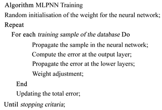
After the training of the MLPNN, thanks for the gradient descent algorithm, the classification process is carried out to generate a lithological map with six classes representing the various rock types found in the study area. A confusion matrix is presented to measure the ability of the classifier in detecting rock types globally found in the study area. The algorithm used for training is given as follows:
3.4. The Architecture on the Keras Platform
The second classification system is implemented using the Keras platform. The same database used in the first classification system was used here, but no pre-processing operation was done. The Keras platform is a toolbox of machine learning algorithms including MLPNN for training and classification. Keras has
![]()
Figure 4. Representation of a MLPNN for the classification of C classes.
the flexibility for code customization. As such personal neural network architecture can be designed from scratch by creating the various layers, fixing the number of neurones in each layer including the hidden layers and one can vary the activation functions from one layer to the next. For the conversion of the database into a proper file format supported by the Keras platform, the Orfeo Tool Box (OTB) library which has the flexibility to provide multiples image processing functions as well as image manipulations tasks was used.
3.4.1. Implementation of the Second MPLNN Using Keras Platform
The MLPNN in the second classification system differs from the first classification system architecture in that; there are 9 layers instead of three layers as in ENVI. These nine layers are organised into one input layer with seven neurones, one output layer with six neurones and seven hidden layers with a total of 64 neurones. The logistic activation function was used as a transition from the first hidden layer to the second hidden layer while the Softmax function was used at the ninth layer also called output layer. The hyperbolic tangent and the logistic function were used for the various transitions between the intermediates layers. Table 1 below clearly described the proposed network configuration. To train the MLPNN, a database was designed using the OTB library as described earlier. Each region of interest (ROI) is a window of 100 × 100 pixels (10,000) pixels. A total of 40,000 pixels is used for training the MLPNN.
The threshold value of the above model in Figure 5 represents the percentage of all the pixels correctly classified in each lithological class. This hyper parameter is fixed as one of the stopping criteria to end the training process of the model and depends on the user but should be at least greater or equals to 50%.
![]()
Figure 5. General architecture of the second classification system.
![]()
Table 1. Description of the network architecture.
3.4.2. Some Hyper Parameters of the Second MPLNN Using Keras
Table 1 illustrates the type and number of layers, the number of neurones per layer and the activation functions used in Keras platform to design the second classification model whose workflow is depicted in Figure 5.
In Table 1, the first column shows the types of layers used in the second neural network including the input for each layer, with hidden (i) for the hidden layer located at the ith position after the input layer and Output for the output layer. The second column shows the number of neurones used per layer including 7 neurones in the input layer, 6 neurones in the output layer, for the six lithological classes and 64 neurones in all the intermediate layers. The third column displays the activation functions used. This includes the Logistic and hyperbolic Tangent (Tanh) functions used at the intermediate layers while the Softmax function which is more suitable for multi-classification tasks is used in the output layer.
4. Results and Discussions
4.1. Results
The presentation of the inputs was done in Section 3.2.2. Table 2 displays a detailed description of the nine input components used where the first column contains the origin of input including PCA, ICA and the OLI sensor while the second and third columns contains the name of feature inputs and the number of each type of feature input respectively. PCA1, PCA2 and PCA3 represents respectively the first, second and third components of the Principal Component Analysis while ICA3, ICA4, ICA5, ICA6 represents the third, fourth fifth and sixth components of the Independent Component Analysis. Band6 and Band7 are simply OLI sensor spectral bands of the Landsat8.
The training data base is made up of six lithological classes extracted thanks to the ROI tool included in ENVI and the geological map of the study area. Table 3 below provides a detailed description of the repartition of the various pixels extracted per lithological class: The training data set represents 80% of the above
![]()
Table 2. Description of the various input bands.
![]()
Table 3. Description of the repartition of the various pixels extracted per lithological class.
mentioned data while the evaluation of the classifier represents 20% of the above data set.
The training data are fed to the MLPNN to generate a lithological map with six classes. The performances of our MLPNN are summarised in the Table 3 and the final lithological map is displayed in the Figure 6.
The second classification system implemented in the Keras platform is having approximately the same performances as depicted in the Table 4 after 1000 iterations. The obtained lithological map is shown in Figure 7.
4.2. Discussion
A critical analysis of the above results is raising the following concerns:
When applied to remote sensing in the lithological multiclass discrimination, the MLPNN does not perform similarly in all the classes involved with a gap in terms of accuracy observed and growing as the number of classes increase. One reason of the following observation can be due to the imbalance distribution of available training data. In addition, the high intra-class variability and the low interclass distance mostly observed in rock lithological classes can also produce these observed discrepancies. Furthermore, the pre-processing phase is a critical phase in that, if it is not well handled, can negatively affect training data by reducing the discriminating power of the descriptors.
Among the various classes, those with low accuracies due to the presence of poorly classified pixels contribute negatively in the overall accuracy which is 53.01% for the first classification system and 49.98% for the second classification system. This situation can be due to the difficulty of the classifier to find suitable
![]()
Figure 6. Updated version of the lithological map from the first classifier.
![]()
Figure 7. Updated version of the lithological map from the second classifier.
![]()
Table 4. Accuracy per class for the second MLPNN classifier in Keras.
discriminating descriptors for those very classes. In fact, different rock units have different susceptibilities to weathering, because of their diverse mineralogical composition, texture, age and rate of erosion, which can lead to different topographic expressions in the field (Yu et al., 2012). A possibility to integrate and run many induction techniques of different natures and configurations on the same training data could enable the identification of a suitable classifier for a given lithological class.
The performances and the visual representation of the lithological map of the two classifiers are almost the same even though in the ENVI platform, pre- processing operations were necessary to get the present results. In Keras however, the flexibility to design and customize our network from scratch is the key point to obtain interesting results with highly noisy data.
The design of the different MLPNN architecture is not yet automated since it is still done with trial and error test. This situation could yield inadequate neural network architecture since the research of suitable architectures in the search space of all the possible configurations is done manually. Therefore, many other configurations are left over.
The design of the two systems has been well spelled out; however, the implementation was based on trial and error. It is believed that for a proper methodology on the design of automated neural network architecture through Neural Architecture Search (NAS) to be obtained, it would go a long way to improve performance. In addition, a deep learning neural network architecture used in conjunction with ensemble method or multi agent system could be explored to address the problem of mixed pixel and reduce the gaps existing between the various lithological classes in terms of accuracy.
5. Conclusion
This research aimed at updating the existing lithological map of the Cameroon’s Center, South and East regions using MLPNN applied to Landsat images. Two different approaches were used for the realization of this objective. The novelty in this research is that we have been able to design two MLPNN with architecture different from the traditional classifiers; with the first implemented on the ENVI platform in conjunction with pre-processing algorithm including Dark subtraction for image correction, PCA and ICA for dimension reduction and band selection as well as feature extraction respectively.
The second architecture implemented on the Keras platform appears to be less complex since the platform allows user customisation. Though the results obtained are almost the same, this model has the advantage that it bypasses the pre-processing phase, thus making it computationally efficient and also robust as it can handle even the noise in the data.