Combined Optimal Stopping and Mixed Regular-Singular Control of Jump Diffusions ()
1. Introduction
Dividend decisions are mainly concerned with financial policies on the payment of cash dividends to shareholders in the present or at a latter date. The decision to issue dividends depends on the firm’s excess cash reserve or profit and its envisaged long term earning capacity. Management is expected to pay out some or all of the cash surplus as dividends if it is not required by the firm. In some instances, excess cash is retained to support future organic growth of the company.
In recent years, several researchers have studied extensively dividend optimisation problems [1] - [10]. This has resulted in various strategies and mathematical models being developed using stochastic control theory [8]. The common dividend payment strategies in literature are band, barrier, threshold and impulse. Scheer, [8] defines the band strategy as one that involves partitioning of state space of the cash reserve in three adjunct sets, A, B and C. Dividends are paid according to the set where the level of cash reserves at time t, and
is located. For example, if
is in A, then the income premium is paid as dividend. The barrier strategy is a special case of the band strategy where the set A consists of only one point, say
and dividends are only paid to shareholders when the amount of cash reserves exceed this point.
Taksar and Zhou [9], examine a dividend optimisation problem of an insurance company with a corporate debt liability such as a coupon bond or amortisation loan. A mixed regular-singular control problem is presented and investigated. The objective is to find a policy that maximises the expected total discounted dividend payout until the time of bankruptcy. In the model, the dynamics of the corporate assets is modelled as a diffusion process with the drift and diffusion coefficients being affine functions of the risk control variable. Taksar and Zhou show that the optimal dividend pay-out policy is to keep the total reserve below a certain optimal level
, distributing the excess as cash as dividends. On the other hand, the qualitative behaviour of the optimal risk management depends on the ratio between the profit
and the liability rate
. When
, then it is optimal not to have reinsurance at all, namely, to take the full risk. On the other hand, if
, then the optimal risk management depends on the current amount of the reserve. There exists
such that the optimal risk
as a function of the reserve x is a strictly increasing function on
, and
for all
.
Zou, etal. [10] present a dividend optimisation problem (for an insurer) with a jump-diffusion risk process in the presence of fixed and proportional transaction costs. Due to the presence of transaction costs, an impulse stochastic control problem is formulated. The stochastic control problem is transformed into a quasi-variational inequality for a second-order non-linear integro-differential equation. Further, the problem is solved under the risk-neutral assumption for the insurer and the value function together with the optimal policy is constructed.
He and Liang [3] investigate optimal financing and dividend control of an insurance company with a proportional insurance policy. The problem is formulated as a mixed singular-regular control problem and solved using dynamic programming. The underlying cash reserve dynamics is modelled using linear Brownian motion [3] considering an optimal dividend and reinsurance strategy of a property insurance company under catastrophe risk.
Empirical studies, however, have shown that the jump-diffusion process reflects better changes that can occur in the level of the liquid assets of an insurance company due to unusual events such as earthquakes and floods [3] [11]. Rare events usually result in huge claims which reduce significantly the amount of cash reserves available to the company. Abrupt changes in the level of the available liquid assets due to unusual events will appear as discontinuities in the cash reserve trajectory. In this study, we extend the problem investigated by Taksar and Zhou [9] by modelling the dynamics of the cash reserve process using a jump-diffusion process. Taskar and Zhou [9] consider a model to maximize the expected total discounted dividend pay-outs for a company with debt liability. In this model, the corporate assets follow diffusion process with diffusion and drift coefficients being affine functions of the risk control variable. Further, we assume that the company has a policy to reinvest a proportion of its excess cash before paying dividends to shareholders. This kind of model is important especially in the context of property insurance. It is important to highlight that only negative jumps are considered in the model under study. The company’s management is faced with a situation where they need to find an optimal business policy that maximises the expected total discounted pay-out. Each business policy is associated with different levels of risk and expected profits. The most basic risk to the company under consideration emanates from claims made by clients on account of the fact that claim sizes vary and their occurrence times are random. This kind of risk is mitigated in the model through reinsurance.
In this paper, we also make the assumption that the company needs positive reserves in order to operate and the company is considered bankrupt as soon as the available cash reserves become negative. Accordingly, we define the bankruptcy time
by
(1.1)
This problem under investigation is unique since it is the first time when a combined optimal stopping and mixed regular-singular control problem involving debt and reinvestment is solved assuming that the dynamics of the underlying cash reserve process is modelled by a jump-diffusion process. In this paper, the researcher chose combined optimal stopping and mixed regular-singular control since it adequately addresses the insurance problem of dividend maximisation and risk minimisation.
The structure of the paper is organised as follows: In Section 2, we present a rigorous mathematical formulation of the general problem on combined optimal stopping and mixed regular-singular control of jump diffusions. Section 3 deals with the application of the general mathematical problem presented in Section 2 to insurance. Section 4 is devoted to a detailed analysis and complete solution of the problem considering different cases of key parameter values such as
and
. In Section 5, we present the numerical examples to illustrate the results obtained in Section 4.
2. Problem Formulation
Consider four components that affect changes in the level of the cash reserves of an insurance company and these are premiums, debt repayments, claims and dividend pay-outs. The first two components namely, premiums and debt repayments are assumed to be deterministic and occur at a constant rate. Dividend payments are determined by the amount of cash reserves available at any given time. Claim sizes vary and occur at random times. A jump-diffusion process is considered in modelling the dynamics of the liquid assets since rare events such as earthquakes and floods can result in huge claims that reduce significantly the amount of liquid assets available to the company. We also take into account the need for the company to mitigate risk arising from its core business through reinsurance. Reinsurance means controlling revenues by diverting a proportion
of all premiums to another company, in which case
fraction of each claim is paid by the other company (Taksar and Zhou, 1998). Suppose
be a stochastic process on a filtered probability space
representing the amount of liquid assets at time t. In this section we begin by considering the general problem formulation on mixed regular-singular control presented by [1] [7]. Let
and
be given continuous functions. Assume the the dynamics of the state
is described by the following equation:
and
is our singular control since
may be singular with respect to the Lebesgue measure
. The process
is non-negative, right continuous and
adapted. Assume also that the performance function is given as follows;
where
and
are given continuous functions,
. Let also
for
be the time of bankruptcy, that is,
. Let
be the set of admissible controls
such that the general equation above has a strong and unique solution. Further, suppose the following condition is satisfied:
where
is expectation with respect to the probability law P given that
. The problem is to find the value function
, the optimal mixed control
and the optimal stopping time
such that;
(2.1)
Theorem 2.1. (Integro-variational inequalities for Combined Optimal Stopping and Mixed Regular-Singular Control of Jump-diffusions)
(a) Suppose there exists a function
such that:
(i)
for all controls
and
.
(ii).
for all
,
.
(iii).
for all
.
(iv).
almost surely on
and
,
.
(v).
is uniformly integrable for all
and
for all
.
(vi). Define the non-intervention region D by;
and suppose
.
Further, assume that for all
, there exists a mixed control
such that
for
(vii)
.
(viii)
for all t,
where
is the continuous part of
.
(ix)
for all jumping times
of
and
(x)
, where
for
. Then
and
is an optimal mixed regular-singular control.
For the proof of (i)-(x) of Theorem 2.1, refer to [1] and [7].
3. Application
We begin by considering four components that affect changes in the level of cash reserves of an insurance company under study and these are: premium payments, debt repayments, client claims and dividend pay-outs to shareholders. The first two components namely, premiums and debt repayments are deterministic and occur at a constant rate. Dividend payments are determined by the amount of cash reserves available at any given time. We also take into account the need for the company to mitigate risks arising from business through reinsurance. Reinsurance means controlling revenues by diverting a proportion
of all premiums to another company, in which case
fraction of each claim is paid by the other company [1].
Let
be a stochastic process on a filtered probability space
representing the amount of liquid assets at time t. We fix a domain
(our solvency region) and let the dynamics of
be modelled by the the following process:
(3.1)
where
is the premium rate and is a positive constant,
is the liability rate,
and
are positive constants,
,
is the reinsurance fraction at time t, y is the initial value of the liquid assets of the company,
is the cumulative dividends paid up to time t,
is 1-dimensional Brownian Motion and
is a compensated Poisson process random measure with intensity
. In our model, we assume that:
(i)
and the compensated Poisson process are independent;
(ii) the company has a policy to reinvest a proportion
of its excess cash; and
(iii) the company pays dividends when
.
where x is the amount of liquid assets at time t,
is a predetermined threshold,
is a proportion of the cash to be reinvested,
and
.
The performance functional for this problem is given by
(3.2)
where
, that is, the first time that the state
reaches the value 0 or below. The problem is to find the optimal stopping time
, optimal control policy
and value function
that maximises the expected total discounted dividend payout. In other words we want
and
such that:
(3.3)
In this model, we will take
as the time at which the company stops payment of dividends to shareholders. The optimal stopping time is determined by the level of liquid assets available.
4. Main Result
In the model, the barrier strategy is used to payout dividends. Dividend payments are only made when the amount of liquid assets or cash reserves available exceed a particular pre-determined level.
Lemma 4.1. Suppose the value of the initial liquid assets is 0, that is,
. Then
,
, for all
and
. The optimal strategy in this case is
where
is arbitrary.
Lemma 4.2. Assume
, then
,
,
and
is arbitrary.
Proof. Suppose
with
and
arbitrary. If
, then it is optimal to immediately distribute the initial cash reserve
sometimes called “take the money and run away strategy”. We have
We note that
. We then want to show that
.
Let
be the state trajectory corresponding to any given control
. From (3.1), we have
where
. The preceding equation can be written as
Integrating LHS gives
(4.1)
where
(4.2)
But
is a supermartingale (See (4.46)). We have
(4.3)
after substituting for
. This implies that
(4.4)
since
and
are constants. We have
(4.5)
Integrating by parts RHS of inequality (4.5), we obtain
We have proved that for
, the optimal dividend payment is the initial wealth or cash reserve y, optimal stopping time
and the optimal policy
.
We now consider the non-trivial case where
and we want to find the optimal stopping time and optimal policy that maximises the expected total discounted dividend pay-out.
Lemma 4.3. Given that
, it is prudent for the insurance company not to do business. It should immediately distribute the initial cash reserve as dividends. The optimal policy in this case is
,
and
.
Proof. Let
where
is to be determined and
. Suppose
, that is, the proportion of reinsurance is 100%. Then the dynamics of the cash reserve is given by
(4.6)
Integrating with respect to t, we have:
(4.7)
We note that
as
since y and
are constants. Hence, when
, the company should not get into business.
Lemma 4.4. Suppose
, then the value function is given by
where
where
(4.8)
(4.9)
(4.10)
(4.11)
(4.12)
where
,
is the amount of cash reserves at time t,
,
and
The optimal strategy in this case is to pay out dividends when
.
Proof
Case 1 (
)
We consider the case
, that is, the company takes maximal risk by retaining all the premiums. The dynamics of the cash reserve is given by
(4.13)
In the absence of dividend payments, the integrodifferential operator of
coincides with its generator given below
(4.14)
Inside the continuation region,
satisfies the following
(4.15)
The non-intervention region D is described by
(4.16)
where
and
.
This implies that
since
and
.
We guess that D has the form
for some
.
Inside D, we must have
. We have
(4.17)
since
. We try a solution
of the form
and substituting into (4.17), we obtain:
We consider
for some constant
. Substituting into the preceding equation, we get:
(4.18)
We note that
and
as
. This implies that the equation
has two solutions
such that
.
Outside D, we require that
(4.19)
Integrating Equation (4.19) with respect to x yields
(4.20)
Hence we put
To find
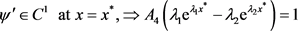
and
, we use the “high contact” principle also called the smooth-pasting condition of singular control which dictates that the value function should be
, in particular at the free boundary
. Now
implies that
. This gives
. We have
Applying the “high contact” principle we have
(4.21)
(4.22)
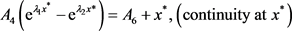
(4.23)
From (4.23), we have
. Dividing through by
, we have
(4.24)
Taking log of both sides of (4.24), we get
(4.25)
From (4.25), we get:
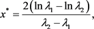
(4.26)
Making
subject of the formula in (4.26), we have
(4.27)
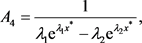
Substituting for
in (4.22) gives
(4.28)
where
is as in (4.27). Substituting for
and
in (4.21) yields
(4.29)
Since the company has an investment policy to reinvest a proportion
of its surplus cash, the optimal strategy is to pay out dividends when
(4.30)
Solving the inequality for x gives
(4.31)
We want to show that
satisfies the conditions of the verification theorem for all the values of
and
.
We have constructed
such that
in D. Outside D, that is for
, we have
. This can be written as:
since at
,
.
We have
which is decreasing in x. From our construction, we have
for
and
for
. Therefore we must have
at
.
Case 2 (
)
We assume
. Inside the continuation region D,
satisfies
. That is
since
. We try a solution of the form
. Substituting it into the preceding equation, we obtain:
In particular, we try a solution of the form
and substitute it into the above equation to get;
(4.32)
In the no jump case, that is,
, the maximum value of a is attained at
(4.33)
Solving for
gives
(4.34)
In the jump case, the value of a is attained at the critical point
.
Differentiating with respect to a and equating to 0 yields
Dividing through byr, we obtain
We let:
(4.35)
Substituting for
in (4.35), we have
We note that
can be written as
Suppose
, then there exists an optimal
such that
(4.36)
We take
as constant. For this value of
, the cash dynamics of the company is given by
(4.37)
We guess that the continuation region is given by
as in case 1. Inside the continuation region, we must have
. This implies that
We try a solution of the form
. Substituting this last equation and simplifying gives
Consider the function
and substitute into the last equation to get;
Define
and  as
as . Therefore, there exists
 .
.
Outside D, we require as in case 1 that . Integrating with respect to x gives
 .
.
We now determine  and
and .
.
 gives
gives 
 . We have

Applying the “smooth fit” principle as in case 1, we obtain
 (4.38)
 (4.39)
 (4.40)
As in case 1, we have
 (4.41)
 (4.42)
where  is as in (4.41). Substituting for
  and
and ![]() in (4.38) yields
in (4.38) yields
![]() (4.43)
(4.43)
![]() (4.44)
(4.44)
![]() (4.45)
(4.45)
where![]() . The optimal strategy in this case is to pay out dividends only when
. The optimal strategy in this case is to pay out dividends only when![]() . We can write the optimal strategy as
. We can write the optimal strategy as ![]() where
where ![]() and
and ![]() are as in (4.44) and (4).
are as in (4.44) and (4).
Theorem 4.1. Fix any initial condition ![]() and consider the problem of maximising the performance criterion
and consider the problem of maximising the performance criterion ![]() over all dividend strategies
over all dividend strategies![]() . The value function
. The value function ![]() is increasing. The following cases provide the solution to the control problem:
is increasing. The following cases provide the solution to the control problem:
(i) If![]() , then
, then![]() ,
, ![]() ,
, ![]() ,
, ![]() for all
for all ![]() and
and ![]() and
and ![]() is arbitrary.
is arbitrary.
(ii). If![]() , then
, then ![]() and
and![]() .
.
(iii). If![]() , then the optimal dividend strategy is to immediately distribute the initial cash reserve as dividends. The optimal strategy in this case is
, then the optimal dividend strategy is to immediately distribute the initial cash reserve as dividends. The optimal strategy in this case is![]() ,
, ![]() and
and![]() .
.
(iv). Suppose ![]() and
and![]() , then
, then![]() ,
, ![]() where
where![]() ,
, ![]() and
and![]() . The optimal strategy is to pay out dividends when the available amount of cash reserves exceed
. The optimal strategy is to pay out dividends when the available amount of cash reserves exceed![]() .
.
Lemma 4.5. Suppose that![]() . Then
. Then ![]() is a super-martingale where
is a super-martingale where
![]() (4.46)
(4.46)
Proof. Let![]() . We have
. We have
![]()
since from (4.46), ![]() ,
, ![]() and
and![]() ,
, ![]() are constants. We conclude that
are constants. We conclude that ![]() is a super-martingale.
is a super-martingale.
5. Numerical Analysis
In this section, we present and analyse the results obtained in Section 4 using numerical examples. The four tables below illustrate the effect of changes in the parameters on the value function, the predetermined threshold ![]() in the barrier strategy, the optimal dividend policy and the reinvestment policy.
in the barrier strategy, the optimal dividend policy and the reinvestment policy.
In Table 1 consider the case when![]() ,
, ![]() ,
, ![]() ,
, ![]() ,
, ![]() ,
, ![]() ,
, ![]() ,
, ![]() ,
, ![]() and
and![]() .
.
In this case, dividends are only paid when the amount of liquid assets at time t is at least equal to 45.5.
In Table 2 consider the case when![]() ,
, ![]() ,
, ![]() ,
, ![]() ,
, ![]() ,
, ![]() ,
, ![]() ,
, ![]() ,
, ![]() and
and![]() .
.
In the case under consideration, the company should pay dividends when the amount of liquid assets at time t is at least equal to 57.8.
![]()
Table 1. Value function versus amount of liquid assets.
In Table 3 if![]() ,
, ![]() ,
, ![]() ,
, ![]() ,
, ![]() ,
, ![]() ,
, ![]() ,
, ![]() and
and![]() .
.
The value function attains the maximum value at 465.9 when the amount of the available liquid assets is at least equal to 153.
Finally, in Table 4 consider![]() ,
, ![]() ,
, ![]() ,
, ![]() ,
, ![]() ,
, ![]() ,
, ![]() ,
, ![]() ,
, ![]() and
and ![]()
In view of the company’s policy, it should only pay dividends when the amount of liquid assets is at least equal to 122.7.
![]()
Table 2. Value function versus amount of liquid assets.
![]()
Table 3. Value function versus amount of liquid assets.
![]()
Table 4. Value Function versus amount of liquid assets.
6. Conclusion
The results in this study have shown that there exists an optimal dividend policy for an insurance company that controls risk through proportional reinsurance, has a debt liability. Liquid assets dynamics is represented by a jump diffusion process and has a policy to reinvest a predetermined proportion of its excess cash. The main empirical findings of the paper are that when the premium rate is less than the liability rate, the company should not get into business and the optimal dividend policy is to immediately pay out the initial cash reserve as dividends to shareholders. While if the premium rate is more than the liability rate, the optimal risk management decisions depend on the current level of the cash reserves. The optimal dividend policy is to pay out dividends as the level of cash reserves is above a predetermined threshold. Further, the use of numerical examples clearly illustrated the effect of changes in the values of the parameters on the value function, the cash reserve threshold and the dividend payouts.