Finite Element Simulation of In-Stent Restenosis with Tissue Growth Model

Jie Cheng, Lucy T. Zhang

Department of Mechanical, Aerospace and Nuclear Engineering, Rensselaer Polytechnic Institute, Troy, NY, USA.

DOI: 10.4236/jbise.2021.142005                

Abstract

In this study, a finite element simulation of in-stent restenosis (ISR) is conducted to simulate the deployment and expansion of a stent in an occluded artery with a contact model and a mechanics-based growth model. A tissue growth model based on the multiplicative decomposition of deformation is applied to investigate the growth of the plaque and artery wall upon the stent’s implantation. Due to the high stresses at the contact points between the stent struts and the tissue, further tissue injury or restenosis is observed. The simulation results show that after the stent deployment, the von Mises stress is significantly larger in the plaque compared to the artery wall, especially in the region that is in contact with the stent. However, the growth of the plaque and artery tends to even out the stress concentration over time. The tissue growth is found to be more significant near the inner wall than the outer layer. A 0.77 mm restenosis is predicted, which agrees with published clinical observations. The features of the artery growth are carefully analyzed, and the underlying mechanism is discussed. This study is the first attempt to apply finite element analysis to artery restenosis, which establishes a framework for predicting ISR’s occurrence and severity. The results also provide insights into understanding the underlying mechanism of in-stent restenosis.

Keywords

Stents, In-Stent Restenosis, Tissue Growth, Finite Element Simulation, Growth Model

1. INTRODUCTION

Cardiovascular disease (CVD) is the leading cause of mortality in the United States in men and women of every major ethnic group. It accounted for nearly 840,768 deaths in 2016 [1]. Coronary artery disease (CAD) is the most common type of heart disease. According to CDC, it claimed 365,914 lives [2] in 2017. Coronary stenting has become a major treatment for coronary stenosis, narrowing a blood vessel leading to restricted blood flow, since its first use in 1986. In the US, 1.2 million patients undergo stent implantations each year [3]. Unfortunately, restenosis, a recurrence of stenosis, often occurs after months or years after the stent implantation. According to [4], nearly one-third of the patients who receive stent implantation require further intervention within six months to reopen stented arteries.

Restenosis is characterized by neo-intima formation, resulting from proliferating medial vascular smooth muscle cells migrating to the intima, and the synthesis of matrix components, mainly collagen, with resultant stenosis and constrictive tissue remodeling [5]. Numerous papers have been published to study the interaction between the stent and the artery. On the one hand, clinical studies are focused on the biological understanding and remedies of restenosis. It has been shown that the biological cause of restenosis could be smooth muscle cell production, endothelial cell abundance, fibroblast growth factors, and so on [6 - 8]. It is observed in in vivo experiments [9] that the vascular wall stress increased immediately after balloon angioplasty. It was also reported that the restenosis rate is closely related to the design of the stents [10]. It is now well-accepted that artery growth is stress-modulated. Therefore, an in-depth study of the stress field in the artery after stent placement becomes necessary. Numerical simulation is undoubtedly a suitable approach to do so.

In one of the early studies, finite element analysis was carried out to examine the maximum principal stress in the stenosed artery caused by two different types of stents [11]. The stent expansion process was not modeled in this simulation, which failed to capture the contacting shear force that an expanding stent could impose on an artery. A similar study was done in [3] with more realistic settings, and the von Mises stress produced by different stents were compared. Some studies were also more focused on fluids flow impacted by the stents [12 - 14], using fluid-structure interaction methods such as the immersed finite element method [15 - 17].

A novel metal stent is modeled as rigid body in [18] where the simulation is mainly focused on the fluid dynamics in the thoracic aorta. A complete stenting system of balloon-stent-plaque-artery was modeled, and the recoil ratio was carefully examined in [19]. An even more realistic stenting process, including the stent insertion and balloon inflation, was modeled in [20]. Except for the idealized models, patient-specific simulations were also reported. The deployment of Bx Velocity stent in the real human coronary artery was simulated in [21], and the influence of the stent thickness was investigated. The effects of six different stents on a patient-specific artery were compared in [22], showing that the numerical simulation can help select stent selection.

All of the previous simulation studies stopped at the calculation of the stress field in the stented artery. In this study, we attempt to simulate the real growth of the artery under the impact of the stent’s deployment. There are various ways to model mechanical-induced growth; for example, the multi-constituent open systems based on the theory of mixtures [23 , 24]. Humphrey and Rajagopal [25] further developed the mixture theory by applying it to flow-induced arterial adaptions. Although it has some successful applications, this approach is quite complicated in implementation and lacks generality. A recent two-dimensional continuum mathematical model of restenosis is proposed in [26] in which diffusion-reaction equations are used for modeling the mass balance between species in the arterial wall.

Unlike the mathematical models cited previously, a mechanical growth model based on the multiplicative decomposition of the deformation was developed [27 , 28]. In this open system thermodynamics framework, an incompatible “growth” configuration was postulated between the material configuration and current configuration, resembling the idea of multiplicative decomposition in the context of finite plasticity, see [29]. This method has been applied in modeling multiple biological structures including arterial wall [30], heart [31], skin [32], brain [33] etc. For relatively new review in this approach, see [34 , 35].

Due to its realisms in presenting tissue growth and simplicity in implementation, the growth model based on the incompatible growth configuration and the decomposition of the deformation gradient into an elastic and growth part is adopted in our study to characterize the long term growth of the arterial wall after implanting the stent. The rest of the manuscript is organized as following: in Section 2, we briefly review the mechanical growth model; in Section 3, the model setup, as well as the geometry, mesh, and boundary conditions are introduced; the results are presented in Section 4, followed by discussions; and finally conclusions are drawn in Section 5.

2. GROWTH MODEL

In this section, we briefly review the mechanical growth model developed in [27 , 28]. The model is described in the aspects of kinematics, equilibrium equations and constitutive equations. This growth model was successfully applied to the simulation of vessel tissue remodeling with residual stress [36].

2.1. Kinematics

The key idea of the kinematics of the growth model is the multiplicative decomposition of deformation gradient $F$ into an elastic part $F_{\text{e}}$ and a growth part $F_{\text{g}}$ . Based on the work in [29 , 37], an intermediate configuration $B_{\text{g}}$ is introduced between the reference configuration $B_0$ and the current configuration $B_{\text{t}}$ . As shown in Figure 1, $\chi$ is the mapping from $B_0$ to $B_{\text{t}}$ , and the deformation gradient $F$ is defined in regular way as $F=\partial \chi /\partial X$ . We assume there exists a decomposition:

$F=F_{\text{e}}\cdot F_{\text{g}}$ (1)

Similarly, the right Cauchy-Green tensor $C$ , velocity gradient $l$ , Piola-Kirchhoff stress $P$ and the second Piola-Kirchhoff (PK2) stress $S$ can be decomposed into elastic and growth parts as well. Let ${\rho }_0$ denote the density in the reference configuration, ${\rho }_{\text{t}}$ and ${\rho }_{\text{g}}$ denote its counterparts in the spatial configuration and the intermediate configuration, respectively. Similarly, define the volume of a material particle in the reference, spatial and intermediate configurations as $\text{d}V$ , $\text{d}v$ and $\text{d}{V}_{\text{g}}$ , respectively. In analogy to $J=\text{det}\left(F\right)$ , define the Jacobians $J_{\text{e}}=\text{det}\left(F_{\text{e}}\right)$ and $J_{\text{g}}=\text{det}\left(F_{\text{g}}\right)$ . The transformations of the volumes become:

$\text{d}v=J\text{d}V\mathrm{,}\text{d}{V}_{\text{g}}=J_{\text{g}}\text{d}V\mathrm{,}\text{d}v=J_{\text{e}}\text{d}{V}_{\text{g}}$ (2)

and

$J=J_{\text{e}}{J}_{\text{g}}$ (3)

Based on the definitions, we have the following density transformations:

${\rho }_{\text{g}}\text{d}{V}_{\text{g}}={\rho }_{\text{t}}\text{d}v\mathrm{,}{\rho }_{\text{g}}=J_{\text{e}}{\rho }_{\text{t}}$ (4)

2.2. Balance Laws

The local form of the balance of mass balances the rate of change of the grown density ${\bar{\rho }}_0$ with a mass source $R_0$ :

${\stackrel{\dot{}}{\bar{\rho }}}_0=R_0$ (5)

Figure 1. The intermediate configuration and the decomposition of deformation gradient.

where the grown density is defined in the reference configuration and can be expressed as ${\bar{\rho }}_0=J{\rho }_{\text{t}}=J_{\text{g}}{\rho }_{\text{g}}$ . For soft tissues, it is typically assumed that the density remains constant upon growth, which means ${\rho }_{\text{g}}=\text{const}$ and ${\stackrel{\dot{}}{\rho }}_{\text{g}}=0$ . So the mass source can be evaluated as $R_0={\bar{\rho }}_0\text{tr}{L}_{\text{g}}$ , where $L_{\text{g}}$ is the growth part of velocity gradient, and can be easily determined by the growth tensor $F_{\text{g}}$ .

The growth process is assumed to be quasi-static, therefore the linear momentum balance is simply:

$\text{div}\sigma =0$ (6)

2.3. Constitutive Equations

An isotropic hyperelastic growth model based on the compressible Neo-Hookean model is used in this study. Denote the Helmholtz free energy as $\varphi \left(C\mathrm{,}{F}_{\text{g}}\right)$ , the PK2 stress and Kirchhoff stress can be evaluated as:

$S=2\frac{\partial \Psi }{\partial C}=2\frac{\partial \Psi }{\partial C_{\text{e}}}\mathrm{<mo>\; :\; </mo>}\frac{\partial C_{\text{e}}}{\partial C}=F_{\text{g}}^{-1}\cdot S_{\text{e}}\cdot F_{\text{g}}^{-\text{T}}$ (7a)

$\tau =F\cdot S\cdot F^{\text{T}}=F_{\text{e}}\cdot S_{\text{e}}\cdot F_{\text{e}}^{\text{T}}$ (7b)

where $S_{\text{e}}$ denotes the elastic part of $S$ . The constitutive moduli $ℂ$ can be obtained by taking the derivative of $S$ with respect to $C$ , and its counterpart in the current configuration can be derived by a push-forward operation:

$ℂ=2\frac{\text{d}S\left(F\mathrm{,}{F}_{\text{g}}\right)}{\text{d}C}=2{\frac{\partial S\left(F\mathrm{,}{F}_{\text{g}}\right)}{\partial C}|}_{F_{\text{g}}}+2\left[\frac{\partial S}{\partial F_{\text{g}}}\mathrm{<mo>\; :\; </mo>}\frac{\partial F_{\text{g}}}{\partial {\theta }_{\text{g}}}\right]\otimes {\frac{\partial {\theta }_{\text{g}}}{\partial C}|}_F$ (8a)

$ℂ=\left(F\bar{\otimes }F\right)\mathrm{<mo>\; :\; </mo>}ℂ\mathrm{<mo>\; :\; </mo>}\left(F^{\text{T}}\bar{\otimes }{F}^{\text{T}}\right)$ (8b)

The detailed derivation of the hyperelastic stress tensor can be found in [38]. It can be seen immediately from Equations (7) and (8) that both the stress and its moduli differ from their usual form only by an additional variable $F_{\text{g}}$ , which is determined independently by the governing equation of the growth. Again, this resembles the concept of finite growth resembles finite strain plasticity in the sense that the basic constitutive equations themselves remain unchanged, however, they are evaluated exclusively in terms of the kinematic quantities of the intermediate configuration.

2.4. Growth Function

To complete the stress and constitutive moduli, the growth deformation tensor $F_{\text{g}}$ must be uniquely determined. It can be either isotropic or anisotropic. In this study, we adopt a simple isotropic form:

$F_{\text{g}}={\theta }_{\text{g}}I$ (9)

where ${\theta }_{\text{g}}$ denotes an internal variable which is often referred to as growth factor. The growth multiplier is 1 in the plain elastic deformation, greater than 1 in growth, and smaller than 1 in atrophy.

To model the evolution of the growth multipliers, the rate of growth multipliers is usually specified as:

${\stackrel{\dot{}}{\theta }}_{\text{g}}=k_{\text{g}}\left({\theta }_{\text{g}}\right)\cdot {\varphi }_{\text{g}}\left(F_{\text{e}}\right)$ (10)

where ${\varphi }_{\text{g}}$ is a growth criteria function to enforce a threshold on the growth, $k_{\text{g}}$ is a weighted function to prevent unlimited growth. ${\varphi }_{\text{g}}$ and $k_{\text{g}}$ are specified with the following forms in [29] with a detailed parameter study:

${\varphi }_{\text{g}}=\text{tr}\left(M_{\text{e}}\right)-M_{\text{e}}^{\text{crit}}$ (11a)

$k_{\text{g}}=\frac{1}{\tau }{\left(\frac{{\theta }_{\text{max}}-{\theta }_{\text{g}}}{{\theta }_{\text{max}}-1}\right)}^{\gamma }$ (11b)

where $\tau$ and $\gamma$ are material constants that are used to control the speed of growth, $M_{\text{e}}$ is the Mandel stress defined as $M_{\text{e}}=C_{\text{e}}\cdot S_{\text{e}}$ , and $M_{\text{e}}^{\text{crit}}$ is the criteria of growth. A local Newton iteration can be used to solve for the growth factor. Applying backward Euler scheme to Equation (10), we have:

${\stackrel{\dot{}}{\theta }}_{\text{g}}=\left({\theta }_{\text{g}}-{\theta }_{\text{g}}^n\right)/\Delta t$ (12)

The residual is evaluated as:

$R={\theta }_{\text{g}}-{\theta }_{\text{g}}^{\text{n}}-\frac{1}{\tau }{\left(\frac{{\theta }_{\text{max}}-{\theta }_{\text{g}}}{{\theta }_{\text{max}}-1}\right)}^{\gamma }\left(\text{tr}\left(M_{\text{e}}\right)-M_{\text{e}}^{\text{crit}}\right)\Delta t$ (13)

To minimize the residual R, we linearize Equation (13) for tangent moduli K:

$K=\frac{\partial R}{\partial {\theta }_{\text{g}}}=1-\left(k_{\text{g}}\frac{\partial {\varphi }_{\text{g}}}{\partial {\theta }_{\text{g}}}+{\varphi }_{\text{g}}\frac{\partial k_{\text{g}}}{\partial {\theta }_{\text{g}}}\right)\Delta t$ (14)

In the local Newton iteration, where the deformation tensor $F$ is known, update the stretch ratio ${\theta }_{\text{g}}$ with ${\theta }_{\text{g}}\leftarrow {\theta }_{\text{g}}-R/K$ . The corresponding growth part of the deformation tensor $F_{\text{g}}$ can be calculated using Equation (9). Consequently the elastic part $F_{\text{e}}$ can be calculated using Equation (1). The elastic stress $S_{\text{e}}$ and elastic constitutive moduli ${ℂ}_{\text{e}}$ can then be obtained using Equations (7) and (8), respectively.

2.5. Baseline Hyperelasticity and Algorithm

In this preliminary work, we use compressible Neo-Hookean as the baseline hyperelastic model since it has been validated in multiple applications [28 - 30 , 37]. But there is no fundamental difficulty preventing other models being used. The compressible Neo-Hookean free energy is written as:

$\Psi =\frac{\lambda }{2}{\ln }^2{J}_{\text{e}}+\frac{1}{2}\mu \left[C_{\text{e}}\mathrm{<mo>\; :\; </mo>}I-3-2\ln J_{\text{e}}\right]$ (15)

The explicit forms of the stress and constitutive moduli can be obtained based on Equation (15):

$S_{\text{e}}=\left[\lambda \ln J_{\text{e}}-\mu \right]C_{\text{e}}^{-1}+\mu I$ (16a)

${\tau }_{\text{e}}=\left(\lambda \ln J_{\text{e}}-\mu \right)I+\mu B_{\text{e}}$ (16b)

and

${ℂ}_{\text{e}}=\left(\mu -\lambda \ln J_{\text{e}}\right)\left(C_{\text{e}}^{-1}\bar{\otimes }{C}_{\text{e}}^{-1}+C_{\text{e}}^{-1}\underset{\_}{\otimes }{C}_{\text{e}}^{-1}\right)+\lambda C_{\text{e}}^{-1}\otimes C_{\text{e}}^{-1}$ (17a)

${ℂ}_{\text{e}}=\left(\mu -\lambda \ln J_{\text{e}}\right)\left({\delta }_{ik}{\delta }_{jl}+{\delta }_{il}{\delta }_{jk}\right)+\lambda {\delta }_{ij}{\delta }_{kl}$ (17b)

where the operation $\bar{\otimes }$ and $\underset{\_}{\otimes }$ between two second order tensors $A$ and $B$ are defined as

${\left(A\bar{\otimes }B\right)}_{ijkl}=A_{ik}{B}_{jl}$ and ${\left(A\underset{\_}{\otimes }B\right)}_{ijkl}=A_{il}{B}_{jk}$ respectively. For more details of the mathematics in con-tinuum mechanics, please refer to [39].

For completeness, we list the specific expressions of Equations (7) and (8) using compressible Neo-Hookean as the baseline hyperelasticity, the detailed derivation can be found in [37]:

$S=\frac{1}{{\theta }_{\text{e}}^2}{S}_{\text{e}}$ (18a)

$\tau ={\tau }_{\text{e}}$ (18b)

and

$ℂ=\frac{1}{{\theta }_{\text{g}}^4}{ℂ}_{\text{e}}-\frac{4}{{\theta }_{\text{g}}^5}\frac{k_{\text{g}}}{K}\Delta t\left(S_{\text{e}}+\frac{1}{2}{ℂ}_{\text{e}}\mathrm{<mo>\; :\; </mo>}{C}_{\text{e}}\right)\otimes \left(\frac{1}{2}{C}_{\text{e}}\mathrm{<mo>\; :\; </mo>}{ℂ}_{\text{e}}+S_{\text{e}}\right)$ (19a)

$ℂ={ℂ}_{\text{e}}+\frac{4}{{\theta }_{\text{g}}}\frac{k_{\text{g}}}{K}\Delta t\left(F_{\text{e}}\bar{\otimes }{F}_{\text{e}}\right)\mathrm{<mo>\; :\; </mo>}\left[\left(S_{\text{e}}+\frac{1}{2}{ℂ}_{\text{e}}\mathrm{<mo>\; :\; </mo>}{C}_{\text{e}}\right)\otimes \left(\frac{1}{2}{C}_{\text{e}}\mathrm{<mo>\; :\; </mo>}{ℂ}_{\text{e}}+S_{\text{e}}\right)\right]\mathrm{<mo>\; :\; </mo>}\left(F_{\text{e}}^{\text{T}}\bar{\otimes }{F}_{\text{e}}^{\text{T}}\right)$ (19b)

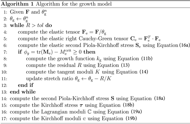
Growth model can be easily implemented within the existing nonlinear finite element framework. In this research the updated Lagrangian formulation is used. Except for the modifications to the Kirchhoff stress and the corresponding constitutive moduli, all the additional computational work it introduces is the iterative solution of the stretch ratio ${\theta }_{\text{g}}$ . Algorithm 1 lists the major part of the algorithm.

3. COMPUTATIONAL SETUP

3.1. Geometry

Promus PREMIER^TM is a relatively new coronary stent designed by Boston Scientific that has a higher strength and less restenosis rate compared to older generations. Here, a 16 mm length model is created with SOLIDWORKS (Dassault Systémes). It is constructed from a cylinder base with a diameter of 2.5 cm and crimped to a catheter with a diameter of 1.055 cm. The thickness of the strut is 0.081 mm. Figure 2(a) shows the planar sketch of the stent, the dimensions are approximated because the original design is not open for public access. Figure 2(b) shows the planar and 3D design of the stent in millimeter. There are 8 struts in the circumferential direction and 13 layers of struts in the longitudinal direction. Notice that there are 4 connectors between two adjacent layers of struts proximally, while there are only 2 elsewhere. The connectors are arranged helically.

The artery is modeled as a tube with a length of 20 mm, shown in Figure 3. The lumen diameter is 3 mm and the wall thickness is 0.8 mm. The plaque is assumed to have a bell-like shape. It is 9 mm long and

the smallest lumen diameter is 1.8 mm. Therefore, the stenosis rate (measured as $1-\frac{D_{\text{blocked lumen}}}{D_{\text{original lumen}}}$) before

stent operation is 40%.

Figure 2. Geometry of the stent. (a) Planar sketch of the stent; (b) 3D view of the stent.

Figure 3. Geometry of the stenosed artery.

3.2. Boundary Conditions

In reality, the stent has to be crimped onto a catheter before inserted into the vessel. After the stent is in place, a folded balloon will be inflated to expand the stent. In this study, we are interested in the interaction between the stent and the artery, besides the expansion of the effective part of the stent is rather uniform [3], therefore the balloon is neglected in our system and the motion of the stent is simplified as prescribed radial displacement.

The simulation is divided into 3 steps: stent crimping, stent expanding, and vessel growth. In the initial stress-free state, the diameter of the stent is larger than the lumen diameter of the stenosed artery. To simulate the crimping process, in the first step, the stent is compressed in the radial direction. The second step is to simulate the expansion of the stent and its interaction with the artery. The stent will expand freely before it reaches the inner wall of the artery. Then the stent will push inner wall of the plaque, expanding the lumen diameter to 3 mm; the last step is the main focus of this study, where we predict the growth of the plaque and artery using the growth model introduced in Section 2.

Table 1 lists the boundary conditions on the stent and the artery in different steps. Because of the periodic nature of the system, only one half of the stent and artery are modeled and a cylindrical coordinate system is used. It is worth mentioning that the radial displacement in the crimping step is −0.431 mm, which means the stent is crimped onto a cylinder with a diameter of 1.8 mm rather than 1.055 mm. This makes no difference because the stent is in elastic phase during the crimping step, it will result with the same state when it gets in contact with the artery.

Table 1. Boundary conditions.

$U_r$ , $U_{\theta }$ , $U_z$ denote the displacements in radial, circumferential, and axial directions respectively. $U_r$ is measured based on the initial state, not the previous step.

3.3. Materials and Mesh

The major component in the stent is 316LN stainless steel. We model it as an elastoplastic material. The material constants are obtained from [40] as listed in Table 2. The material of the artery is described with the compressible Neo-Hookean as mentioned in Section 2. The material constants and growth parameters are obtained from [30], as listed in Table 3. The material property of the plaque is changing with its development. We assume it is in the beginning of the calcification stage, when it is much stiffer than the healthy artery. Since there is no experimental data for the growth parameters, we adopt them from [29]. This set of parameters has not been calibrated with clinical results; it only describes the growth qualitatively. The growth exponent and adaption speed are relatively high in order to accelerate the growth. The growth criterion is low, which makes growth more evident. Finally the maximum growth factor is set to bound the growth in a reasonable range.

In this analysis, the displacement of the stent is prescribed, therefore it is modeled with shell element to simplify the computation. A total of 7261 elements are used. The artery is modeled with C3D8 element since the geometry is simple and material is compressible, 25,560 elements are used.

4. RESULTS AND DISCUSSIONS

4.1. Crimping

The diameter of the outer surface of the stent is 2.662 mm in stress-free state. It should be crimped onto a 1.055 mm-diameter catheter before being inserted into the artery. However, since the crimping process is in the elastic range, we only need to crimp it to 1.8 mm, which is as wide as the stenosed artery, so that it does not penetrate the artery before the expansion begins. Figure 4 shows the von Mises stress in the artery-stent system at the end of the crimping process. At this point, the artery is stress-free, while the stent is not. From this point on, the stent and the artery are in contact.

4.2. Expanding

As the stent continues expanding, the plaque will be pushed to the artery wall. The goal of the operation is to recover the lumen diameter to 3 mm. Figure 5(a) and Figure 5(b) present the geometry of the artery-stent system and the von Mises stress in the artery at the end of the expansion process, respectively.

Table 2. Material constants of the stent.

Table 3. Material constants and growth parameters of the artery.

Figure 4. Von Mises stress in the artery-stent system at the end of crimping process.

It can be seen that after the stent operation, the plaque is significantly compressed, and the inner wall of the vessel becomes flat. The von Mises stress in the healthy tissue is negligible compared to the plaque. The contact area can be clearly observed based on the stress field. Maximum stress in the plaque indicates the danger of the rupture.

4.3. Growth

The growth process starts after the expansion. In our model, the Mandel stress is the source of growth,

Figure 5. Geometry and Von Mises stress at the end of expansion process. (a) Geometry of the artery-stent system; (b) Von Mises stress in the artery.

Figure 6 shows the Mandel stress in the artery during the growth process. As expected, the Mandel stress is gradually decreased because of the growth of the tissue. At the final state, the Mandel stress in the whole artery becomes 0, which indicates the end of the growth. Restenosis is also observed in this figure: the plaque “bounces back” towards the inner direction. The amount of the growth is shown in Figure 7. Starting from the initial state where $\theta =1.0$ , the growth factor increases to the maximum. The growing area expands from the plaque to the vessel wall. The growth in the plaque is much faster than the healthy tissue. However, because the growth is bounded, the lumen diameter of the artery is still larger than the pre-procedure state in Figure 4.

To visualize the restenosis quantitively, we look at the change of the lumen diameter from the pre-procedure state to the final stable state after restenosis as shown in Figure 8. At normalized time $t=2$ , the lumen diameter is pushed to 3 mm. Interestingly, the lumen diameter continues increasing for a short period of time, expanding to 3.2 mm before it starts to decrease. This is due to the compressible nature of the material: in the early stage of the growth, the stress generated from the compression is not large enough to hold the growth. After this point, the restenosis starts to develop, until the growth is terminated by the criterion, which is the so-called biological equilibrium. The final lumen diameter is 2.23 mm, therefore, the loss due to the restenosis is 0.77 mm and the net gain of the stent operation is 0.43 mm. The restenosis rate is 64.2%, which is quite severe but reasonable given the problem setup.

To compare the growth at different locations in the artery, the growth factors at 5 points along the radial direction in the middle of the artery wall are sampled. It can be seen from Figure 9, the growth is weakened from the inner wall to the outer wall as expected. The relationship between the distance to the inner wall and the growth factor is highly nonlinear. The results show the change in the near-wall area is

Figure 6. Mandel stress in the artery during the growth: (a) The initial state; (b) t = 100; (c) t = 200; (d) t = 300.

Figure 7. Growth factor in the artery during the growth: (a) The initial state; (b) t = 100; (c) t = 200; (d) t = 300.

not as significant as in the middle. Moreover, the change of the growth factor over the normalized time is also highly nonlinear. This is likely due to the sensitivity of the growth model. Unfortunately only a limited number of parameter studies are done in literature to perform a quantitate analysis. The qualitative findings are found to be consistent with clinical observations.

Figure 8. Lumen diameter.

Figure 9. Growth factors along the radial direction: Point 1 to 5 are distributed uniformly from the inner wall to the outer wall.

5. CONCLUSIONS

Restenosis is a common side effect of the stent procedure which is caused by the tissue growth. Clinical study has been carried out for years but the mechanism of the growth is still not clear. Researchers in the field of computational mechanics have only been involved in the area of biological growth recently yet there are already plenty of outcomes. The stent procedure has been studied in many previous papers. However, in this study, we push the study forward by applying a stress-induced growth model to the post-procedure artery. The growth of the artery tissue is investigated. Qualitatively, it is found that the maximum growth factor is mostly concentrated in the area that is in contact with the stent, since it is where the stress is the highest. This implies that the goal of the design of the future stents should be focused on reducing stress concentration. Quantitively, the lumen diameter of the post-procedure artery is found to be re-narrowed from 3 mm to 2.23 mm, which is reasonable based on clinical observations.

It can be seen from this study that finite element analysis is a promising tool to study some of the complicated biological growth that in vivo investigations are difficult to apply to. However, there are also unsolved problems: first, in order to characterize the growth more realistically, experiments must be done to find the proper growth parameters; second, the growth is assumed to be isotropic, which is not necessarily true because we know the vessel is highly anisotropic. More sophisticated growth model may be required to capture the anisotropy.

Conflicts of Interest

The authors declare no conflicts of interest regarding the publication of this paper.

References

[1]	American College of Cardiology. AHA 2019 Heart Disease and Stroke Statistics.
[2]	Centers for Disease Control and Prevention. Heart Disease Facts.
[3]	Gu, L.X., Zhao, S.J., Muttyam, A.K. and Hammel, J.M. (2010) The Relation between the Arterial Stress and Restenosis Rate after Coronary Stenting. Journal of Medical Devices, 4, Article ID: 031005. https://doi.org/10.1115/1.4002238
[4]	Llyod-Jones, D., Rosamond, W., Flegal, K., Friday, G. and Furie, K. (2009) Heart Disease and Stroke Statistics—2009 Update: A Report from the American Heart Association Statistics Committee and Stroke Statistics Subcommittee. Circulation, 119, 480-486.
[5]	Buccheri, D., Piraino, D., Andolina, G. and Cortese, B. (2016) Understanding and Managing In-Stent Restenosis: A Review of Clinical Data, from Pathogenesis to Treatment. Journal of Thoracic Disease, 8, E1150. https://doi.org/10.21037/jtd.2016.10.93
[6]	Nakamura, N., Torii, S., Tsuchiya, H., Nakano, A., Oikawa, Y., Yajima, J., Nakamura, S., Nakano, M., Masuda, N., Ohta, H., et al. (2020) Formation of Calcified Nodule as a Cause of Early In-Stent Restenosis in Patients Undergoing Dialysis. Journal of the American Heart Association, 9, e016595. https://doi.org/10.1161/JAHA.120.016595
[7]	Shlofmitz, E., Iantorno, M. and Waksman, R. (2019) Restenosis of Drug Eluting Stents: A New Classification System Based on Disease Mechanism to Guide Treatment and State-of-the-Art Review. Circulation: Cardiovascular Interventions, 12, e007023. https://doi.org/10.1161/CIRCINTERVENTIONS.118.007023
[8]	Giacoppo, D., Alfonso, F., Xu, B., Claessen, B.E.P.M., Adriaenssens, T., Jensen, C., Pérez-Vizcayno, M.J., Kang, D.-Y., Degenhardt, R., Pleva, L., et al. (2020) Paclitaxel-Coated Balloon Angioplasty vs. Drug Eluting Stenting for the Treatment of Coronary In-Stent Restenosis: A Comprehensive, Collaborative, Individual Patient Data Meta-Analysis of 10 Randomized Clinical Trials (Daedalus Study). European Heart Journal, 41, 3715-3728. https://doi.org/10.1093/eurheartj/ehz594
[9]	Saito, N., Mori, Y. and Komatsu, T. (2020) Inuence of Stent Exibility on Artery Wall Stress and Wall Shear Stress in Bifurcation Lesions. Medical Devices (Auckland, NZ), 13, 365. https://doi.org/10.2147/MDER.S275883
[10]	Müller, M.D., Gregson, J., McCabe, D.J.H., Nederkoorn, P.J., Bart van der Worp, H., de Borst, G.J., Cleveland, T., Wolff, T., Engelter, S.T., Lyrer, P.A., et al. (2019) Stent Design, Restenosis and Recurrent Stroke after Carotid Artery Stenting in the International Carotid Stenting Study. Stroke, 50, 3013-3020. https://doi.org/10.1161/STROKEAHA.118.024076
[11]	Lally, C., Dolan, F. and Prendergast, P.J. (2005) Cardiovascular Stent Design and Vessel Stresses: A Finite Element Analysis. Journal of Biomechanics, 38, 1574-1581. https://doi.org/10.1016/j.jbiomech.2004.07.022
[12]	Gay, M., Zhang, L.T. and Liu, W.K. (2006) Stent Modeling Using Immersed Finite Element Method. Computer Methods in Applied Mechanics and Engineering, 195, 4358-4370. https://doi.org/10.1016/j.cma.2005.09.012
[13]	Gay, M. and Zhang, L.T. (2009) Numerical Studies of Blood Flow in Healthy, Stenosed, and Stented Carotid Arteries. International Journal for Numerical Methods in Fluids, 61, 453-472. https://doi.org/10.1002/fld.1966
[14]	Gay, M. and Zhang, L.T. (2009) Numerical Studies on Fluid-Structure Interactions of Stent Deployment and Stented Arteries. Engineering with Computers, 25, 61-72. https://doi.org/10.1007/s00366-008-0105-2
[15]	Zhang, L.T. and Gay, M. (2008) Imposing Rigidity Constraints on Immersed Objects in Unsteady Fluid Flows. Computational Mechanics, 42, 357-370. https://doi.org/10.1007/s00466-008-0244-8
[16]	Cheng, J., Yu, F.M. and Zhang, L.T. (2019) OpenIFEM: A High Performance Modular Open-Source Software of the Immersed Finite Element Method for Fluid-Structure Interactions. Computer Methods of Engineering and Sciences, 119, 91-124. https://doi.org/10.32604/cmes.2019.04318
[17]	Liu, W.K., Liu, Y.L., Farrell, D., Zhang, L.T., Wang, S.X., Fukui, Y., Patankar, N., Zhang, Y., Bajaj, C., Lee, J., Hong, J., Chen, X. and Hsu, H. (2006) Immersed Finite Element Method and Applications to Biological Systems. Computer Methods in Applied Mechanics and Engineering, 195, 1722-1749. https://doi.org/10.1016/j.cma.2005.05.049
[18]	Chaparro-Rico, B.D.M., Sebastiano, F. and Cafolla, D. (2020) A Smart Stent for Monitoring Eventual Restenosis: Computational Fluid Dynamic and Finite Element Analysis in Descending Thoracic Aorta. Machines, 8, 81. https://doi.org/10.3390/machines8040081
[19]	Wei, L.L., Leo, H.L., Chen, Q. and Li, Z.Y. (2019) Structural and Hemodynamic Analyses of Different Stent Structures in Curved and Stenotic Coronary Artery. Frontiers in Bioengineering and Biotechnology, 7, 366. https://doi.org/10.3389/fbioe.2019.00366
[20]	He, R., Zhao, L.G., Silberschmidt, V.V. and Liu, Y. (2020) Mechanistic Evaluation of Long-Term In-Stent Restenosis Based on Models of Tissue Damage and Growth. Biomechanics and Modeling in Mechanobiology, 19, 1425-1446.
[21]	Gijsen, F., Migliavacca, F., Schievano, S. and Socci, L. (2008) Simulation of Stent Deployment in a Realistic Human Coronary Artery. Biomedical Engineering Online, 7, Article No. 23. https://doi.org/10.1186/1475-925X-7-23
[22]	Auricchio, F., Conti, M., De Beule, M., De Santis, G. and Verhegghe, B. (2011) Carotid Artery Stenting Simulation: From Patient-Specific Images to Finite Element Analysis. Mechanical Engineering and Physics, 33, 281-289. https://doi.org/10.1016/j.medengphy.2010.10.011
[23]	Bowen, R.M. (1976) Theory of Mixtures, Volume 3 of Continuum Physics, Mixtures and EM Field Theories. Academic Press, Cambridge, Chapter 2, 1-127. https://doi.org/10.1016/B978-0-12-240803-8.50017-7
[24]	Rajagopal, K.R. and Tao, L. (1995) Mechanics of Mixtures. World Scientific, Singapore.
[25]	Humphrey, J.D. and Rajagopal, K.R. (2003) A Constrained Mixture Model for Arterial Adaptations to a Sustained Step Change in Blood Flow. Biomechanics and Modeling in Mechanobiology, 2, 109-126. https://doi.org/10.1007/s10237-003-0033-4
[26]	Escuer, J., Martínez, M.A., McGinty, S. and Pena, E. (2019) Mathematical Modelling of the Restenosis Process after Stent Implantation. Journal of the Royal Society Interface, 16, Article ID: 20190313. https://doi.org/10.1098/rsif.2019.0313
[27]	Cowin, S.C. and Hegedus, D.H. (1976) Bone Remodelling I: Theory of Adaptive Elasticity. Journal of Elasticity, 6, 313-326. https://doi.org/10.1007/BF00041724
[28]	Kuhl, E., Menzel, A. and Steinmann, P. (2003) Computational Modeling of Growth. Computational Mechanics, 32, 71-88. https://doi.org/10.1007/s00466-003-0463-y
[29]	Himpel, G., Kuhl, E., Menzel, A. and Steinmann, P. (2005) Computational Modeling of Isotropic Multiplicative Growth. Computer Modeling in Engineering and Sciences, 8, 119-134.
[30]	Kuhl, E., Maas, R., Himpel, G. and Menzel, A. (2007) Computational Modeling of Arterial Wall Growth: Attempts towards Patient-Specific Simulations Based on Computer Tomography. Biomechanics and Modeling in Mechanobiology, 6, 321-331. https://doi.org/10.1007/s10237-006-0062-x
[31]	Oomen, P.J.A., Holland, M.A., Bouten, C.V.C., Kuhl, E. and Loerakker, S. (2018) Growth and Remodeling Play Opposing Roles during Postnatal Human Heart Valve Development. Scientific Reports, 8, Article No. 1235. https://doi.org/10.1038/s41598-018-19777-1
[32]	Zollner, A.M., Buganza, T.A., Gosain, A.K. and Kuhl, E. (2012) Growing Skin-Tissue Expansion in Pediatric Forehead Reconstruction. Biomechanics and Modeling in Mechanobiology, 11, 855-867. https://doi.org/10.1007/s10237-011-0357-4
[33]	Wang, L.M. and Kuhl, E. (2020) Viscoelasticity of the Axon Limits Stretch Mediated Growth. Computational Mechanics, 65, 587-595. https://doi.org/10.1007/s00466-019-01784-2
[34]	Menzel, A. and Kuhl, E. (2012) Frontiers in Growth and Remodeling. Mechanics Research Communications, 42, 1-14. https://doi.org/10.1016/j.mechrescom.2012.02.007
[35]	Kuhl, E. (2014) Growing Matter: A Review of Growth in Living Systems. Journal of Mechanical Behavior of Biomedical Materials, 29, 529-543. https://doi.org/10.1016/j.jmbbm.2013.10.009
[36]	Cheng, J. and Zhang, L.T. (2019) Simulation of Vessel Tissue Remodeling with Residual Stress: An Application to In-Stent Restenosis. International Journal of Smart & Nano Materials, 10, 11-27. https://doi.org/10.1080/19475411.2018.1529002
[37]	Goktepe, S., Abilez, O.J. and Kuhl, E. (2010) A Generic Approach towards Finite Growth with Examples of Athlete’s Heart, Cardiac Dilation, and Cardiac Wall Thickening. Journal of Mechanics and Physics of Solids, 58, 1661-1680. https://doi.org/10.1016/j.jmps.2010.07.003
[38]	Cheng, J. and Zhang, L.T. (2018) A General Approach to Derive Stress and Elasticity Tensors for Hyperelastic Isotropic and Anisotropic Biomaterials. International Journal of Computational Methods, 15, Article ID: 1850028. https://doi.org/10.1142/S0219876218500287
[39]	Holzapfel, G.A. (2000) Nonlinear Solid Mechanics: A Continuum Approach for Engineering. Wiley, Hoboken.
[40]	Saraswat, P., Chinnakonda, M. and Baillargeon, B. (2016) Living Heart Human Model: Cardiovascular Stent Deployment and Cardiac Cycle Simulation. Journal of Medical Devices, 10, Article ID: 030945. https://doi.org/10.1115/1.4033869