1. Introduction
Other way to introduce quagnetic field is generalized four forces which directly indicate existence and form of the quagnetic field. Newton and Coulomb laws for forces are treated as four forces for space-time continuum. Hence four forces of Newton law are obtained using Euler-Lagrangian [1] equation of motion where a particle is in gravitational field. The four forces are obtained via four accelerations. Those are simplified by replacing Christoffel term with potential containing parallel displacement term [2]. This is expressed as change in potential per its unaltered original potential. Alternatively the four potentials are defined using the action function hence the four forces are further simplified. It provides generalized four forces equation for gravitating system. Not much in need of present work, however for the sake of symmetry, the electromagnetic Coulomb law four forces are obtained similar to gravitating system. Finally the required new field is authenticated as quagnetic field with space-time medium resistance
for gravitoquagnetic system. Here the symbol “
” is chosen for quagnetic field and
is for quagnetic induction. Interestingly for gravitated system, the new field other than quagnetic field is obtained based on new induction term having only time components. i.e. the induction
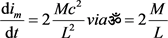
appeared as rate of change of mass current and relates with  as
as  Where “
 ” is like inverse permeability type constant and it is
pronounced as “oum”. The  equals to
thus
equals to
thus  where
is Einstein constant and k is gravitational constant G.
where
is Einstein constant and k is gravitational constant G.
For electromagnetic system the new field other than magnetic field based on new induction term
is observed. The new induction is derived as rate of change of current and it relates with
as
, where
is permeability. For existence of any coexisting pair of fields as polar and axial vector fields, a permanent fundamental particle should exist in nature. For electromagnetic and gravitoquagnetic systems respectively a charge and a mass particle are present in nature. The new fields other than required here in present work are based on gravitoquagnetic super curvilinear induction term
and based on electromagnetic super curvilinear induction term
. The super curvilinear word is used because their coexisting field members are quagnetic curvilinear field and magnetic curvilinear field respectively. But here two permanent fundamental particles at their rest positions to emerge quagnetic and to emerge magnetic fields forever are absent or are not known yet. Or for brevity an argument can be put forward about having three coexisting natural vector fields as linear, curvilinear and super curvilinear for each permanent fundamental particle.
Other alternative way is to recognize quagnetic field using energy-momentum tensor for macroscopic system [3] and it is treated as being continuous. Maxwell equations for Electromagnetic system in integral form and differential form for the stationary states and the time-varying fields are bases of extended Maxwell equations for gravitoquagnetic system. The first and second extended Maxwell equations are as under
and
and their differential forms are as
and
.
In which the first is based on Gauss law and the second is based on argument “gravitating monopole does not exist” as in the case of magnetic field respectively. The term
is introduced as gravitational induction. Remaining
two extended Maxwell equations of gravitating system are proved [4] theoretically and suggested as under

where im is mass currents similar to Ampere law and ig is quagnetization current. Here all the electromagnetic laws like Ampere law, Faraday law, Lenz law etc. are suggested equally applicable for gravitoquagnetic system. For that purpose, charge, charge current, electric potential, electromagnetic resistance etc. are needed to be replaced by mass, mass current, gravitated potential, gravitoquagnetic resistance etc. respectively. Thus for convenience, all the electromagnetic laws, equations etc. are renamed for gravitoquagnetic system by adding “extended” word before electromagnetic terminology. For example Faraday law is applicable to gravitoquagnetic system as extended Faraday law.
Differential form of the same is given as

where
is mass current density.
Extended Faraday law for fourth gravitating extended Maxwell expression leads to
and as
where
is flux of quagnetic induction and
is gravitating potential. Its differential form is
Experiments to prove aforesaid expressions are not possible on earth. Because to induce one s−1 quagnetic induction approximately 1027 kg/s mass current is needed. It can be possible in planetary system or in galactic movements. Astronomical data may help in said requirement.
2. An Alternative Way to Introduce the Quagnetic Field “⊚” Part (I)
The four accelerations [2] are characterized using equation of motion of a particle in gravitational field. The standard Euler-Lagrangian equation [1] for the same is as
,
where
and
are four velocities,
are four accelerations, four forces are given as
Here covariant form of motion of particle is given as
and
The gkl plays role of potential of the gravitational field and its derivative
determines the field intensity.
For
thus
for
. Comparing this expression [5] with the term
, the
potential turns as constant potential as
. Recalling
and putting
and
, the four forces are presented as
The action function for gravitating system is given as
. Because for gravitating system, the curvilinear field is not available yet thus inspiring from electromagnetic action [6]
, gravitating action [7] is obtained as
The term
defines gravitational field flux
, after omitting limits; the action expression is as under
and it is also expressed as
, thus
Hence the four forces are presented as with positive sign as
Here
is included and
is multiplied by
.
If
is not included and
is not multiplied by
, gravitational four forces would be appeared as below with minus sign
This minus signed expression of force is matched with nonrelativistic approximation [8] result.
This is four forces general expression for gravitating system. For electromagnetic system, the expression [9] of motion of charge is given as
,
is electromagnetic field [10] given as
Where
are electromagnetic potentials. Similarly for gravitating equation of motion can be obtained as
is gravitating field defined as
where
are gravitating potentials. By putting
and
, here multiplier
of
is not included, the referred expression appears as
,
where
and
, thus
,
where
and
is unity under the condition
. So,
.
Integrating over flux immerging surface
. Thus
,
Recalling
and replacing
by mG, the gravitating four forces
would be
.
By using the expression
and
, the electromagnetic four forces are
.
The four velocities [9]
and
are unit less and those are defined as
and
for
.
So,
and
are simplified as
and
.
Here if multiplier
of
is included for
,
appears with negative sign. Further the action function for gravitating system is chosen as
hence gravitational potential is obtained as
.
It leads to gravitational four forces as
Finally the electromagnetic four forces can be expressed with 4π as below
It looks satisfactory having 4π at denominator for coulomb four forces but it also creates compulsion to include 4π in Newtonian four forces.
The interactions between two particles having masses or charges at
or at cdt distances for gravitating and electromagnetic system respectively lead to operator or quotient transformation as
. Realizing
are not continuous and limits of
do not tend to zero. Further the initial points of
distances are assumed at the zero. Thus
turns as
. Thus the
and
are further simplified as
and
.
Generalized expression of four forces for both the electromagnetic and gravitoquagnetic systems may be defined as
where
represent type of particle m or Q and both particles
and
must be same type either mass particles or charge particles.
refer constants which are known as permittivity, permeability etc. i and j run from 0 to 3 for time and space coordinates respectively. Here in aforesaid expression for electromagnetic four forces,
is omitted. Because inclusion of
compulsorily for both the systems exhibits the Newton force with multiplier
. For
; the
represent linear vector fields as electric field E or as gravitational field g. Thus E matrix and g matrix can be exhibited as under.
Total Coulomb law matrix and field are
Total Newton law matrix and field are
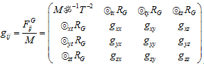
where
and
both turn as cT for time coordinate and for that corresponding field is denoted with suffix (t).
and
both turn as L for space coordinates and field is denoted with suffix
. The
and 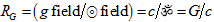 represent space time medium resistance. For only space coordinates
;
and
total nine components to each are equivalent to E field and g field respectively. For only time component
,
and
represent space time medium resistance. For only space coordinates
;
and
total nine components to each are equivalent to E field and g field respectively. For only time component
,
and 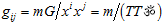 total one component to each is equivalent to E field and g field respectively. Here unexpected new inductions are characterized as Q/TT and m/TT. Those are appeared for both the systems respectively. Remaining mix component combination for
,
and
,
and
;
and
total one component to each is equivalent to E field and g field respectively. Here unexpected new inductions are characterized as Q/TT and m/TT. Those are appeared for both the systems respectively. Remaining mix component combination for
,
and
,
and
;
and 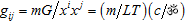 total six components to each are equivalent to E field and g field respectively. Here known H = Q/LT magnetic field and expected
quagnetic field are appeared as to maintain symmetry among their systems and to support the said statement of present work.
total six components to each are equivalent to E field and g field respectively. Here known H = Q/LT magnetic field and expected
quagnetic field are appeared as to maintain symmetry among their systems and to support the said statement of present work.
2.1. Two New Fields
Two new inductions Q/TT and M/TT for both the systems are obtained in four forces matrix as in relation with electric and gravitational field as under
and 
By Rearrangement technique [4] the linear vector field expressions
and
the curvilinear vector field expressions
and  can be obtained. Similarly by Rearragement technique the curvilinear field expressions
and
can be obtained. Similarly by Rearragement technique the curvilinear field expressions
and  can be converted into so called super curvilinear expressions
and .
.
So, new electromagnetic field is
and new gravitoquagnetic field is
.
The magnetic [11] and quagnetic inductions of curvilinear vector fields are defined in proportion of looped charge current and looped mass current as
and  respectively. Whereas the new inductions are found in proportion of rate of change of loop currents as
and
. Thus new fields can be expressed as
respectively. Whereas the new inductions are found in proportion of rate of change of loop currents as
and
. Thus new fields can be expressed as
and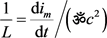 .
.
It leads to
 and
.
and
.
2.2. Relation of New Fields with Chistoffel Symbol and Riemann Tensor
Above expression defines gravitoquagnetic new induction
is as energy emerged from area of given volume and it might be appeared as
Induction
For electromagnetic new induction
can be predicted as
times energy emerged from area of given volume.
The gravitoquagnetic new field
is defined using expression
as,
![]() .
.
Thus the new field
nearly admits itself as Chistoffel symbol. And square of the new field
represents component of Riemann tensor.
If for the electromagnetic system, magnetic field as curvilinear field is not known, the new electromagnetic field
might be defined using expression
as
where
and
are electric potentials and
is the electric Christoffel symbol. Term
or
might be known as component of electromagnetic curvature tensor [7] or electromagnetic Riemann tensor.
2.3. Gravitational New Field and Einstein Equations
At last, by putting approximate values of
and
for macroscopic gravitating system, expression of super curvilinear vector field ![]() is might be suggested as
is might be suggested as
![]() .
.
Components of Riemann curvaturetensor [7] [12] is might be suggested as
![]() and
and
![]()
represents components of Riemann tensor. If in expression ![]() ॐ is replaced by
ॐ is replaced by ![]() it turns as
it turns as
It looks similar to Einstein field equations
where
is component of Riemann tensor and
is Einstein constant
![]() . Concluding aforesaid, it can be suggested that presently introduced so called super curvilinear gravitating expression can be appeared as somewhat look alike Einstein field equations. This might be theoretical authentication of existence of new fields other than quagnetic field as super curvilinear vector fields for gravitoquagnetic as well electromagnetic systems.
. Concluding aforesaid, it can be suggested that presently introduced so called super curvilinear gravitating expression can be appeared as somewhat look alike Einstein field equations. This might be theoretical authentication of existence of new fields other than quagnetic field as super curvilinear vector fields for gravitoquagnetic as well electromagnetic systems.
3. An Alternative Way to Introduce the Quagnetic Field “⊚” part (II)
Analogies of gravitoquagnetic and electromagnetic system are as under,
![]()
Multiplying last two equations of left side with E and H respectively for electromagnetic system and combining those and similarly multiplying last two equations on right side with g and
respectively for gravitoquagnetic system and combining those. One gets further analogies using relation
as
![]()
Applying volume integration and using Gauss’ theorem for second term at right side, surface integral vanishes for both the systems and relations are obtained as
![]()
Now analogy is obtained for closed systems consisting of particles and fields which are conserved. Here first term represents energy of field itself and thus
![]()
This present finding concludes that the curvilinear field component to the linear gravitational conventional field is appeared for compensating the said “completeness”. Similar approach is reflected in the Lorentz invariant theory of gravitation (LITG) [13] [14] [15] [16] as combination of linear gravitational vector field with the gravitational torsional field [17]. In the present study, the quagnetic induction Bg (torsional in LITG), strength
, quagnetization and constant ![]() are extracted from Einstein field equations and extended Einstein field equations. This gravitational torsional field is second component of gravitational field acting on the mass in translation or rotating motion. This torsion field (quagnetic induction = Bg) is essential to satisfy the Lorentz covariance principle for gravitational field potentials. The torsion field
and the gravitational field strength
are being part of gravitational tensor and the energy density of gravitational field. i.e. the gravitational tensor
are extracted from Einstein field equations and extended Einstein field equations. This gravitational torsional field is second component of gravitational field acting on the mass in translation or rotating motion. This torsion field (quagnetic induction = Bg) is essential to satisfy the Lorentz covariance principle for gravitational field potentials. The torsion field
and the gravitational field strength
are being part of gravitational tensor and the energy density of gravitational field. i.e. the gravitational tensor
and vector of energy flux density [13] [14] [15] [16] as
.
Which is also called Heaviside vector [17]. Comparing these two quantities the torsion field
and the gravitational field strength
with the present quantities energy density of field
![]()
and Poynting vector
for gravitating system respectively, one may conclude that the torsional part of energy density is equalized as ![]()
The torsional part of Heaviside vector is equalized with Poynting vector as
.
This leads to gravitational inverse permeability ![]() and one the most important relation as
and one the most important relation as
![]() analogous to electromagnetic relation
. More analogies are appeared as
analogous to electromagnetic relation
. More analogies are appeared as
![]() curvilinear field – induction relation
.
curvilinear field – induction relation
.
![]() curvilinear energy density component
curvilinear energy density component
curvilinear gravitational field
.
Thus torsion field
is appeared merely as quagnetic induction (often called gravito magnetic field) of quagnetic curvilinear field strength
with gravitational inverse permeability![]() . The point is that to comply with the
. The point is that to comply with the
principle of Lorentz Covariance about the gravitational field potentials, compulsion necessity of inclusion of torsion field (quagnetic induction field Bg) leads to rational essentiality of “completeness” i.e. “A vector field can be specified almost completely, if its divergence and curl are given everywhere in space” and thus that authenticates presently introduced statement i.e. “Every natural linear vector field coexists with its counterpart natural curvilinear vector field”.
Thus electromagnetic energy momentum tensor form is as
, where
Similar form is adopted for gravitoquagnetic system (gravi electromagnetic) from general energy momentum tensor form given here as
is some function of quantity q and here the quantities q are the components of the four potential of the field. Hence similar form as electromagnetic energy momentum tensor can be used for gravitoquagnetic system as
where
,
is four potentials of the gravitoquagnetic field, ![]() Constant 4π is not applicable for gravitoquagnetic system however for time being it is retained to hold symmetry with electromagnetic system.
Constant 4π is not applicable for gravitoquagnetic system however for time being it is retained to hold symmetry with electromagnetic system.
Variation of Λ appears as
, where
Therefore
For contra variant components
To symmetrized the tensor
, the quantity
is added and within the variation of gravitoquagnetic total action
Coefficients of
must be zero and in absence of masses, the mass current density
, thus
. It leads to
and hence finally the energy momentum tensor for gravitoquagnetic system is obtained as
.
The components
. Components of the tensor
in terms of gravitational field intensity (g) and quagnetic field intensity (
) are easily verified as
goes with energy density i.e.
![]() ,
,
go with components of Poynting vector i.e.
![]()
and the space components
go with three dimensional tensor components i.e.
![]()
![]()
or in general
![]()
is might be called Maxwell stress tensor for gravitoquagnetic system similar as LITG gravitational stress energy tensor [13].
Thus component of stress energy tensor [13] are given as
.
where ![]() for
term and
for
term and
![]() for other terms
for other terms
![]() ,
,
![]() ,
,
![]() ,
,
![]() ,
,
![]() ,
,
![]()
Gravitomagnetic vector
= Gravitational momentum density
In electromagnetic system the energy densities are given as
similarly for the gravitoquagnetic system the energy densities are given as
![]()
where gravitational linear field induction
looks similar as
.
Because
, but
. Here
ensures the new field is quagnetic field
and its induction is quagnetic induction
. so, for
![]()
can be obtained. Where ![]() is gravitating inverse permeability dimensionally
connected with quagnetic field and its induction is
is gravitating inverse permeability dimensionally
connected with quagnetic field and its induction is ![]() similar to magnetic induction
for stationary state.
similar to magnetic induction
for stationary state.
The expression ![]() is dimensionally written as
is dimensionally written as ![]() and for quagnetization effect,
and for quagnetization effect, ![]() term should be added. The quagnetization
is induced in object while it is facing external quagnetic field
, similar as magnetization M is induced in object surrounded by external magnetic field H. Thus expression becomes
term should be added. The quagnetization
is induced in object while it is facing external quagnetic field
, similar as magnetization M is induced in object surrounded by external magnetic field H. Thus expression becomes![]() . This has been derived by adding extra action term (interaction between field and matter) in Einstein field equation in associated article quagnetic field part (I) [4].
. This has been derived by adding extra action term (interaction between field and matter) in Einstein field equation in associated article quagnetic field part (I) [4].
4. Three Quantities
,
and ![]()
Three quantities (
= quagnetic induction,
= quagnetic field and ![]() = quagnetic inverse permeability) are in need to be clarified simply. Whatever names of these three properties, here those are defined as
= quagnetic inverse permeability) are in need to be clarified simply. Whatever names of these three properties, here those are defined as
Acknowledged as torsional field = gravito magnetic (induction) field = quagnetic (induction) field = time dilation = cogravitational field etc. Origins of this gravitational curvilinear vector (induction) field are
Any mass moving linearly or rotating or spinning is liable to produce
. And any distortion in space time fabric via motion of mass is also equally liable to produce
. This is obeying the relation
![]()
for translation motion of mass, where Im is mass current and L is distance from trajectory of mass and the point at where the induction is measured. Direction of such induction is rotating (curving) and it is perpendicular to the propagating direction of mass. For rotating circular motion
is obeying the relation
![]() or
or![]() .
.
Numerical value of ![]() makes the value of induction down to tiny. It means, for inducing one s−1 time dilation, one needs about 1027 (kg/s) mass current to flow. Direction of such induced
field is perpendicular to the plane of circulation of mass and parallel to the axis of circulation.
is diverged fast following 1/r rule as it moves far from the rotating disc.
makes the value of induction down to tiny. It means, for inducing one s−1 time dilation, one needs about 1027 (kg/s) mass current to flow. Direction of such induced
field is perpendicular to the plane of circulation of mass and parallel to the axis of circulation.
is diverged fast following 1/r rule as it moves far from the rotating disc.
The parent mass Mp (any planet or star or galaxy) is given as
, mi are the masses of n atoms (in parent mass Mp, trillions of atoms are localized) here Mp is supposed to at rest. Within the parent mass Mp, atomic electrons with having masses are orbiting their own nuclei and thus producing quagnetic or torsional or gravito magnetic inductions
. Thus due to moving charges anti parallel tremendous magnetic induction exists but here it is not in picture. Accumulation of unidirectional (oriented in same direction) inductions
are not the case of interest here but inductions
oriented and emerged in all the directions having almost same probable magnitudes of inductions are targeted. Logic is to retain effect of rotating masses associated with orbiting electrons. For example, within our earth, total weight of all electrons is about 1.594 × 10²¹ kg. (roughly 17.5 × 1051 electrons). All electrons are rotating with speed of about less than or equal to one percent of speed of light in atomic orbits. How can we neglect effect (torsion or quagnetic induction = Bg) of this much mass
with tremendous rotating speed
. This much revolving mass matters
noticeably plus the speed of mass matters gigantically as a whole! Fortunately planes of rotations of all the electrons are not aligned otherwise the total quagnetic induction (torsion effect) produced by these electrons associated masses (1.594 × 10²¹ kg) would be resulted into gigantic gravitational acceleration (only in the pinpointed direction of Bg) for the earth
Yes
.
5. Origin of Gravity
Conventionally, the gravity is believed as an output of merely an amount of gross mass which might be stationary or moving (not up to relativistic level) heavy parent mass. i.e. the amount of gravity does not bother about effect of dynamics of all orbiting electron masses at atomic level within the parent mass nor bother about motion of parent mass as a whole. The conventional “g” is given as
In present study, gravity is suggested as an accumulation effect of motion of all orbiting electron masses at atomic level inside heavy parent mass. Really this is not negligible amount of quagnetic (torsional) induction! Here nuclei (protons + neutrons) are assumed stationary due to extremely polarized positon of center of mass between electrons and nuclides of each atom.
Invariably rotating mass associated with orbiting atomic electrons (mass is driven by electromagnetic force) cause large amount of quagnetic induction or time dilation even if the parent planet mass is at rest. This might be the origin of gravity i.e.
Gravitational acceleration = velocity of light × induction (
) or say
.
Here a stationary large parent mass (any planet or star or galaxy) is emerging quagnetic or gravito magnetic induction field through its two dimensional surface area from three dimensional (spatial) volume of the sphere. Production of Bg for single orbiting electron mass is
![]() .
.
is rotating mass current associated with orbiting electron.
For total electron mass of whole planet,
is given as.
![]() ,
,
The me is mass of single electron, a0 = Bohr radius. Total mass of all electrons of planet Me = Mp/3855.6 where 3855.6 is derived as proton and neutron mass contribution per each electron for planet i.e. For one electron mass, total 2.1 proton mass is adopted in intra-atomic (limited up to n = 1 and n = 2 orbits) charge particle distribution and thus (mass of proton + 1.1 × mass of neutron) = 2.1 mass of proton = 2.1 × 1836 mass of electron = 3855.6 mass of electron.
Now gravity at surface of an electron is given conventionally as gone elec= (Mass of one electron me/square of electron radius L0) G, i.e.
Now gravity due to (present idea) rotating electron owing Bohr radius a0 as
![]() , thus
, thus
,
where
is mass current of one electron, v is the velocity of that electron in first orbit, n is the principle quantum number,
is Bohr radius,
is the radius of electron,
is the fine structure constant as
and
Finally the relation
is obtained via constant
. The partial part
of full constant
is appeared due to g is measured at different distances like at Bohr radius
and like at (surface of an electron) radius of electron L0 from the center for the present formula (![]() ) and for the conventional formula (
) respectively. Moreover in the present formula, electron is moving with speed of v at with
radius and in the conventional formula the speed of electron at surface is obviously c thus one more
is added to complete the constant
.
) and for the conventional formula (
) respectively. Moreover in the present formula, electron is moving with speed of v at with
radius and in the conventional formula the speed of electron at surface is obviously c thus one more
is added to complete the constant
.
Here one serious point, out of relevant topic and out relevancy of this article can be raised as: Any stationary (Heavy in mass) positive or negative charge equivalent to electronic charge is asking (as a heavy host particle) escape velocity for rotating charge particle (lighter victim particle) as vesc = c. This same distance between host and victim particle is considered as minimum possible radius of host particle, no one can dare to think deeper than this said radius, because we cannot even experimentally measure nor theoretically allow vesc > c. As a result proton radius is overestimated as
.
In general, it is a fact that a charge equivalent to electronic charge and being a host heavy particle (proton or antiproton) always offers vesc = c for lighter oppositely charged victim particle (electron or positron) between distance 0.84 × 10⁻¹⁵ meter to 0.87 × 10⁻¹⁵ m. This distance is accepted the ultimate radius of host particle! Alternatively if only charge is considered (irrespective of host mass) of a host particle, it offers vesc = c at 2.817 × 10⁻¹⁵ m for victim particle, hence radius of host is assumed 2.817 × 10⁻¹⁵ m. For example, protium, deuterium and tritium (successive heavier nucleus) respectively offer vesc = c for orbiting electron at larger and larger distances (>0.87 × 10⁻¹⁵ m). In contrary considering muonic hydrogen where 200 times heavier (compared to electron) negative muon is orbiting proton with shorter wavelength compared to electron. The equation
allows muon to have shorter
. Similarly the equation
allows muon to have shorter vesc = c orbit (thus,
the radius of host proton is recorded as 0.841 × 10⁻¹⁵ m). Here
is fine structure constant and
is minimum wavelength of victim particle (muon). This suggests clearly that if one is experimenting to rotate heavier and heavier particle in place of muon, shorter and shorter radius of proton (<0.841 FM) will be (illusionary observed) recorded. There is no limit, i.e. heavier and heavier mass of rotating victim particle forces to observe smaller and smaller radius of host particle (here proton).
Back to the present article: Now to extend this one electron gravity relation up to planetary system, one has to make some replacements as under
,
![]() ,
,
is mass of all electrons of considered planet thus the ratio
It leads to
or
This (Bg)planet is a large quantity! If this is not considered to relate to gravity, on what account this much quagnetic induction and related energy due to rotating masses associated to orbiting electrons of big masses (planets, stars, galaxies) likely to forfeit?
First of all the calculated “g” using idea of
and the empirical “g” are found almost same. The ratio for all planets is
, thus
![]()
Here
amount is might be analogous to effective surface area of an atom from which the quagnetic induction emerges. It is given as
Actual calculations of the ratio
and ratio
of some planets are given as Table 1.
It leads to effective atomic radius (I = 2.4156 × 10⁻⁷ m) of an emerging surface.
![]()
Table 1. Calculation of inverse of effective surface area of an atom and ratio of calculated and empirical value of gravity of some planets.
Naturally, this amount is constant for all planets’ atomic radius for emerging surface. Alternatively, using Gauss law for gravitational system, the conventional relation
can be obtained. Here conventionally mass of planet Mp is accepted as main cause of gravity. Total gravitational field is exerted from perfect spherical surrounding area (
) is somewhat due to presence of mass Mp at center and space time medium property gravitational constant G.
Now, in accord to the present idea, quagnetic field (Bg) is accepted as main cause of gravity. This suggests that instead of a stationary mass as a main cause of gravity, total effect of moving masses of rotating electrons within that stationary mass is accepted as a main cause of gravity.
This is rather finer approach to expose the effect of that stationary mass in detail. i.e.
![]()
is suggested as main cause of gravity in place of mass. In other words: The net flux through any closed surface surrounding a quagnetic field source Bg is given by BgGnew. i.e. Gauss law formula
can be obtained.
Here it is predicted that the total gravitational field is exerted from perfect spherical surrounding area (
) is somewhat due to presence of (Bg)total = constant × Mp and new space time medium property Gnew = G/constant,
![]() .
.
Naturally “g” of any planet can be calculated using aforesaid formula i.e.
. Here the rate of time i.e. (TBg)mass in vicinity of mass compared to flat space time rate of time i.e. (TBg)flat decides the gravity. If a test particle owes rate of time (TBg)test, only attraction between the same is possible. Because negative (TBg) is not existed. Here Newton force exerted between them is
,
![]() ,
,
here Im is constant for
and m = mass of electron. In short, if electrons are not driven by electromagnetic forces to orbit (with associated masses) their nuclei at atomic level as component units of the parent mass, intuitively suggestive a big statement (I really afraid) might be given as: gravitation properties might not be existed. Philosophically, if electromagnetic force is not driving masses associated with orbiting electrons around nuclei, gravitational attractions amongst masses are might be under dilemma. When mass of orbiting electron in atom as an unit component for parent mass is in act, movements of parent mass as a whole is a different story and not to match the present case for producing induction field
.
At last, still I am not sure about to declare stationary elementary or sub- elementary particles (having zero energy of vibration, rotation and excitation and with zero velocity) are gravity less entities, because this matter is dealing with truly big thing.
6. Electro-Magnetic-Gravito-Quagnetic (EMGQ) Combined System
In whole the Universe, trillions of stars, debris, matter clouds are active radiator of electromagnetic activities. Such activities are resulted owing movements of charges. Charges are bound to carry inbuilt masses with having identical movements. Amount of such inbuilt masses is noticeably high or nearly comparable to mass of visible Universe. Movements of this much mass emerge tremendous amount of quagnetic or torsional or gravitoquagnetic type field. If this much gravitoquagnetic activities are not considered entangled (attached) or accommodated within the electromagnetic activities, where would one forfeit this much gigantic energy of gravitoquagnetic activities? Because the same gigantic energy is not appeared or not detected anywhere in any form, that is why it forces to think about the merger of electromagnetic activities with gravitoquagnetic activities as one unit like Electro-Magnetic-Gravito-Quagnetic (EMGQ) combined system in favor of conservation. This helps to debit gigantic energy of gravitoquagnetic activities due to moving inbuilt masses of charges on account of EMGQ combined system.
More specifically, it is established fact that any charge is never been at rest and never been free from associated mass, and in the case of heavy parent mass (planets, stars, galaxies), accumulation of such electrons associated rotating masses owing gigantic value of quagnetic activities as a whole. Now during production of electromagnetic wave by any natural or artificial technique or coincidences, the mass associates with charge are forced to move in identical manner with respect to charge (no choice for associated inbuilt mass). If movements of charges are responsible for production of electromagnetic wave, simultaneously identical movements of associated masses are being responsible to produce entangled gravitoquagnetic (gravi electromagnetic) wave (not the propagating wrinkles in space time as a distortion in space time fabric due to movements of heavy uneven distributed masses or their densities and those masses are losing momentum to collide)! It is expected that the entangled gravitoquagnetic wave (means it coexists with electromagnetic wave) propagates within the electromagnetic wave sharing same propagation axis and sharing same planes of component vibrations. Detailed efforts are as given below.
6.1. Duplex and Quadruplex Symmetry and Helicity for Combined EMGQ System
Duplex symmetry (EM-system) ensures the free-field Maxwell equations are unchanged by the transformation regarding altered E, B fields. Similarly duplex symmetry (GQ-system) suggests that the free-field Maxwell equations of gravitoquagnetic system are unchanged [18] by the transformation regarding altered g and Bg fields.
The present quadruplex symmetry (linear combination of two duplex symmetries of two concerned systems with coefficients = 1) promises that the free-field Maxwell equations of combined EMGQ system (linear combination of Maxwell equations of both the considered electromagnetic and gravitoquagnetic systems with coefficients = 1) are unchanged by the transformation regarding altered E + g, B + Bg fields. Detailed work is given as under.
The electromagnetic free Maxwell equations are in natural units and in addition whenever the equations in natural units are required in MKS units, both the said equations are shown with equality sign. Maxwell equations are as
The gravitoquagnetic free Maxwell equations are as
The introduced electromagneticgravitoquagnetic (EMGQ) combined free Maxwell equations are as addressed as linear combination of fields with coefficients = 1.
To hold symmetrical units for Maxwell equations for electromagnetic and gravitoquagnetic combined system, the Linear Combination of Maxwell Equations (LCME) can be adopted as having
leads to
where
.
leads to
where
.
leads to
where
and
.
Leads to
where
and
.
Thus Maxwell equations for combined EMGQ system with identical units (in form of electromagnetic units) are as
Where
Where
.
Where
and
.
Where
and
.
It suggests that the Maxwell equations are general. Instead of presently used two systems if one adds more up to n-systems,
and
formulated as
system 1
system 2
system 3 + … +
system n and similarly for
interestingly the gravitoquagnetic system is perfectly placed fit in the Maxwell equations for combined systems by means of symmetry and linearity. It can be marked without doubt that the presently introduced statement “Every natural linear vector field coexists with its counterpart natural curvilinear vector field" is authenticated.
The standard duplex symmetry formulas for electric field E and magnetic field B are
and
to make the electromagnetic free Maxwellian equations unaltered when those applied in place of E and B respectively.
Similarly the duplex symmetry [18] formulas for gravitational field g and quagnetic induction field Bg
and
make the free Maxwellian equations for gravitoquagnetic system unaltered [18] when those applied in place of g and Bg respectively.
For the present EMGQ combined system, the introduced quadruplex symmetry formulas for electric field E, magnetic field B, gravitational field g and quagnetic induction field Bg are as
.
These make the “free combined Maxwellian equations” unaltered when those applied in place of E and B as well G and Bg respectively for Electro MagneticGravito Quagnetic (EMGQ) combined system.
This quadruplex symmetry can be extended for transverse vector potentials for Electromagnetic system as choosing
and
as well
and
for gravito quagnetic systems in natural units These new potentials for both the systems are satisfying relation given under
By choosing the Coulomb gauge one gets plane wave equations for both the systems as C = 0 and
or
Now the introduced potentials are satisfying the Maxwell equations for both the systems by choosing transverse components as
and
Naturally, the duplex symmetries of individual systems are in need of conserved quantity often called helicity. For the purpose of total helicity (helicity of combined EMGQ system), the quadruplex symmetry in infinitesimal form should be approached like
Now using Noethers [19] theorem, two individual helicities per volume (for electromagnetic system it is wb2/m3) are obtained using routine process considering MKSA system.
and
, c = velocity of light
and
Here the name of MKSA unit for gravitoquagnetic helicity density is tentatively chosen as “Meber2” = “Mb2” = Meter4/sec2. Thus 1 weber = (Kilogram/Coulomb) × Meber. For the total helicity density, introduced combined potentials are treated as
.
Thus total density is associated to the total helicity is given as
and
To hold symmetrical units for different helicities of electromagnetic and gravitoquagnetic systems, the Linear Combination of Invariant Helicity (LCIH) can be adopted as
,
and
thus
If one changes the coefficients values as
and
thus
In short, concluding the aforesaid as a whole, Electromagnetic duplex symmetry leads to conserved quantity EM-Helicity (
) as
Gravitoquagnetic duplex symmetry leads to conserved quantity [18] GQ-Helicity (
) as
Combined Electro Magnetic Gravito Quagnetic (EMGQ) quadruplex symmetry leads to conserved quantity EMGQ helicity as
Or using the Linear Combination of Invariant Helicity
(LCIH),
and
, thus
These potentials are gauge-independent quantity. Referring physical content of both the systems via Maxwell equations, all four potentials
and
satisfy the wave equations and so there are plane waves travelling at the speed of light. Again referring single plane wave
and
are perpendicular to the wave vector k and each potential is orthogonal to first nearest neighbor potential and anti-parallel to the second nearest potential. Here
and
point toward the direction of propagation of combined wave vector k. more specifically, here to accommodate four transverse field components (B, E, Bg and g) to vibrate in xy plane (wave vector K lies in z direction) with four helixes which projections are being periodic transverse components of four fields (E, H, g,
). At initial state, +x, +y, −x and −y directions are allotted to potential A, C, Ag and Cg respectively. In short, all four fields’ resultant successive cross products travel in z-direction simultaneously sharing same wave vector k and alternatively sharing all four quarters of same xy plane or x-y axis to vibrate their field components.
6.2. Orthogonality
Orthogonal functions like f(x) and g(x) are to follow routine integration check as below and have to satisfy certain four conditions like
Now for two individually orthogonal sets (f, g) and (h, i) the checks are
,
here
it means
.
,
here
it means
.
For individually zero valued integrative checks of two sets of orthogonal functions without any doubts lead to
. But those do not guaranty about all possible sets (having two functions per each set) necessarily or essentially mutually orthogonal functions. Yes, dot product of sets (having two orthogonal functions to each set) is completely vanishing.
Detailed orthogonality among chosen fields E, B, g, Bg is given as
From the definition [3] of densities μ and ℯ, μ/m = ℯ/q where m is mass and q is charge. It leads to
where
are fluxes of both the densities respectively,
and
are space
time medium resistance (impedance). The formula
suggests the relation
. Formulas
lead to two equations with dot products as
further lead to
.
Now it is known that
and
. These free space perpendicularities cause individual zero valued dot products for
,
,
and
four equalities of the fields.
Thus
turn as
and
with inequalities
and
Finally
,
,
and
perpendicularities authenticate the probabilities of coexistence of electromagnetic and gravitoquagnetic activities as a single unit having quadruplex symmetry and four helixes with combined helicity and mechanical invariant properties like energy density, Pointing-Heaviside vector etc.
6.3. The Energy Densities
The Lagrangian densities for the free electromagnetic system (i.e.
) and free gravitoquagnetic system (i.e.
) can be given using electromagnetic scalar field tensor property FijFij and gravitoquagnetic scalar field tensor property QijQij but thus both the Lagrangian densities are not appearing as duplex symmetry individually. For that duplex symmetry purpose, coupled electromagnetic dual field tensor
GijGij to the FijFij (i.e.
)
and coupled gravitoquagnetic dual field tensor
RijRij to the QijQij (i.e.
)
are to be needed. In case of these duplex symmetries of both the systems, now by using Noethers [19] theorem i.e.
and
time-translation invariance of the Lagrangian densities leads to the conserved quantities as energy densities for both the systems as
for electromagnetic duplex symmetry and
![]()
for gravitoquagnetic duplex system [18]. In light of aforesaid discussion, the combined EMGQ conventional Lagrangian density can be given as
.
Now the Lagrangian density for quadruplex symmetry of combined EMGQ system would be chosen as
.
Similarly the time-translation invariance of this combined Lagrangian density lead to the conserved quantity as energy density for both the systems as a whole via Noetherʼs theorem i.e.
As
![]()
This is also conserved total energy density, having quadruplex symmetry and time translation invariant property.
6.4. Poynting-Heaviside Vector
Poynting
and Heaviside (
) combined vector is
.
Combined vector (Poyting Heaviside vector) for EMGQ (Electro Magnetic Gravito Quagnetic) system is given as
This is suggesting that the transverse components E, G, g and
of EMGQ system are vibrating individually in perpendicular manner to first neighbor components (having total two first neighbors) and vibrating in antiparallel manner to second neighbor (having total one second neighbor) component and orthogonal to the direction of EMGQ wave. i.e.
Intensities and amplitudes of gravitoquagnetic components (
) are very less compared to electromagnetic components (
) but those are invariably to travel together! Thus Photon and graviton (in sense of only gravitoquagnetic wave packet = graviton) are travelling together with no special separate identity (i.e. photon is forever in compulsion to coexist with graviton)! But obviously only dominant components are noticed forever! On the other hand the graviton (gravitoquagnetic wave packet) is not in compulsion to coexist with photon when large mass moves under gravitational potential difference or under external accelerative forces. Actually in this process gravitoquagnetic waves are produced and such superimposed accumulation of gravitoquagnetic waves (wave packet) is graviton.
6.5. Role of EMGQ System in Pair Production and Light Ray Deviation (Gravitational Lensing)
6.5.1. Pair Production
Refereeing pair production via Gamma rays, conventionally it is established that a Gamma ray photon carries minimum energy equals to two electrons mass and passes near nucleus, electron and positron are appeared with equal positive masses and with opposite charges to compensate the photon energy and to compensate charge neutrality of photon respectively.
The present combined EMGO system defines the same story of pair production as: Conventionally total energy density of electromagnetic wave by incorporating electric and magnetic components is given as
.
Total energy of electromagnetic wave is given by (may be related to components of gravity)
.
As the stronger and stronger source of electromagnetic wave (i.e. higher and higher the amount of oscillating charges and higher and higher the frequency of oscillating charges) is gradually used, the energy En(mass) (which is in form of variable frequency hence related to components other than electromagnetic type) as well the energy density En(EM) have to enhance on equal footage. Here energy density En(EM) of electromagnetic component part can be enhanced via two parameters, first is variable amount of oscillating charge and second is via enhancing frequency (causes enhanced field flux EL2) of the wave. The energy density of electromagnetic component part would be
This is enhanced via increment in electric and magnetic components density via shortening the wavelength. While electric and magnetic amplitudes are only enhanced when charge of oscillating poles of the source are enhanced at given distance! Whereas En(mass) is enhanced via increment of frequency of wave. The electric amplitude has limit to enhance itself up to super saturated E-field value for given source charge q (charge of electron) as
.
Otherwise Gauss law equality results in to inequality as
, here q is the charge of an electron and
is radius of electron. It means that the electric amplitude cannot be allowed to be bigger than maximum possible field amplitude emerged by given source charge q (charge of electron). In other words, maximum amplitude of electric field components (positive and negative side) are expected to appear not larger than the field size at surface of +q and –q at any time of pair production. But wavelength has no limit to decrease. More decrement of wavelength cause harder gamma rays and at last resulted into more kinetic energies for the pair after spending required energy to produce masses of positron and electron.
Now at this stage only wavelength is being shorter and shorter as stronger (vibrating capacity) the source is used while electric amplitude is forcefully truncated as to match charge of electron. i.e. En(EM) only cares about electrical things means cares about energy density related to only electrical components, it is not reactive to foreign gravity. In case of production of electromagnetic wave via electron or proton jumps down between two concern energy levels at atomic or nuclear level respectively, the electrical components are dependent to the amount of charge (generally electron or proton) which has to jump down. The En(mass) is taking care about energy related to how fast the charges are oscillating (i.e. frequency of oscillations) or (as alternate option) energy related to the energy gap of two concerned energy levels (between which electron or proton has to jump down) at atomic or nuclear level.
In vicinity of large positive center (nucleus), electrically super saturated positive radial components (likely to transform into positive charge by having sufficient electric field flux EL2 to match
, thanks to adequate En(mass) for providing required
) of electromagnetic (actually EMGQ) gamma wave repels itself from nucleus. In similar pattern electrically super saturated negative radial components of electromagnetic (actually EMGQ) gamma wave find attraction from nucleus. Thus both the positive and negative components (forced by nucleus to separate and transformed in to the particles by having sufficient afore said requirements) are diverted from the main stream wave vector K and travel in opposite directions to each other. Question is how to furnish equal positive masses for both electron and positron? From where the equal positive masses associated with both the charges of the said pair are appeared? Electrical components are not to carry mass or mass related energy. Thus somebody (in form of field components which are likely to transform in to equal masses) has to take responsibility for equal distribution of mass to the pair and should be strongly associated (entangled) to the electric field components with same frequency and phase. Straight answer is gravitational super saturated components (likely to transform into positive mass + me =gL2/G having sufficient gravitational field flux gL2 to match gL2 = meG thanks to adequate En(mass) for providing
) of gravitating field (g) of gravitoquagnetic wave as a part of EMGQ wave. Those are responsible to provide masses to the pair via entangled gravitational field components with electrical field components. Magnetic and quagnetic components are being cause of spins of the pair elements.
6.5.2. Gravitational Components are not Fully Reactive (Responsive) to Gravity
Above discussion concludes that the Gamma ray photon is invariably combined with Gamma ray graviton. The graviton part carries at least minimum energy equals to two electron masses and consists of gravitational and quagnetic wave components. Normally these gravitational components being parts of gravitoquagnetic wave which is fragment of total EMGQ wave are not fully reactive (sensitive to gravity) to its own source gravity as well gravity of foreign object. In support to this statement, Einstein shift event stands well as: A 5000 Å (λoriginal) visible light (originated from Sun) is shifted 0.01 Å (
) towards the red in influence of its own source (sun) potential GMsun/Rsun. A 5000 Å radiation’s electric components are obviously unreactive to the gravitational potential of the Sun. Here the gravitational components (because this is EMGQ radiation) find themselves responsible to work against the potential by sacrificing some energy in form of frequency (increment in wavelength). So very tiny amount of sacrificed work against gravitational potential of the Sun by radiation (λoriginal) is given as
. Thus said reactivity of gravitational components towards the source gravity is negligible. The reason is that the gravitational components and entangled electrical components are not in capacity to transform them in to gravity reactive as well electricity reactive (sensitive) single particle (electron with mass or positron with mass). It is because of having insufficient frequency (Energy for gravitoquagnetic part and energy density for electromagnetic part of EMGQ wave) to match transformation of gravitational wave components to mass and having insufficient electrical positive potential on the surface of Sun to transform electrical components in to charges. In short, no scope of pair production causes tiny reactive property of gravitational components towards gravity (by sacrificing tiny amount of frequency of emerged radiation from moderate star mass, the Sun). The electrical components are not associated with mass (in absence of probability of pair production) so such unreactive electrical components are not in compulsion to be dragged with mass. This leads to direct or indirect lack of reactiveness of electric components to gravity of their own source as well gravity of foreign object. Outcome of this paragraph is: Any EMGQ (conventionally electromagnetic) radiation with whatever the amount of capacity to match transformation in to mass (pair production), response of that radiation towards the gravity is in proportion to that said amount of capacity. i.e. higher the energy (frequency) of that radiation causes higher the loss of radiation energy. Now bear with me for one paragraph for a little side tracked topic.
6.6. Any Electromagnetic (Actually EMGQ) Radiation Can Escape from Black Hole
In light of Einstein’s formula
for Einstein shift (Redshift), things become obvious like “It is irrational to announce that even an electromagnetic radiation cannot escape from the Black hole”.
Here is the proof 1: The Einstein’s formula
leads to have shift
Math_564#towards the red using maximum potential
(Black hole). It means having an
(E.q.
Math_568#) wavelength radiation can come out (emerge) from black hole source with having
(E.q.
Math_571#) Å wavelength. So greater than or equal tohalf of the initial energy is sacrificed by radiation but the electromagnetic radiation can always be entitled to escape from black hole!!!! It suggests that, in case of ‘pair production competent gamma ray’, that gamma ray may be transformed in to said pair and now the fully transformed masses from their concerned field components as the pair (electron with mass and positron with mass) are not in position to escape from the Black hole. In short a radiation having fractionally transformed gravitational field components in to fractional mass (or in to polarization of mass) will lose its energy on behalf of reactivity towards the gravity. It is in proportion to amount of fractionally transformed gravitational components in to mass but can escape from the Black hole. Matter (Fully sensitive to gravity) having velocity even v = c (if possible) cannot escape from Black hole, but due to partial sensitivity of gravitational vector components towards the gravity, EMGQ (conventionally electromagnetic) wave obviously can escape from the Blackhole. The sensitivity of gravitational vector components towards the gravity is directly in proportion of energy of that radiation consists of gravitational and electrical vector components.
Here is the proof 2: The Einstein formula
for gravitational lensing clearly indicates that the deviation angle
for victimized light ray (EMGQ wave) is maximally one degree for gravitational potential of heavy object equals to
. Having such gravitational potential for the heavy object categorized itself as Black hole. So Black hole deviate the victimized light ray by amount of only one degree. Here victimized light ray (EMGQ wave) slightly deviates from its path. The light ray (EMGQ wave) is not completely captured by black hole while it travels in vicinity of that heavy object which holds gravitational potential
.
Now back to the article topic: Neutral Photon part carries positive and negative electrical field components of wave. As the combined system [(Photon + Graviton) may be noticed as Graphoton)] passes near nucleus; masses of electron and positron are appeared with equal positive mass incorporating and for compensating Graviton energy (
). The masses are present on behalf of fully transformed gravitational field components of wave. The charges of same electron and positron are appeared with opposite signs to compensate the charge neutrality of photon and to exist on behalf of fully transformed electrical field components of wave.
6.7. Gravitational Lensing
Secondly the gravitational lensing means deviation of electromagnetic wave (actually EMGQ wave) in vicinity of great gravitating object is conventionally accepted due to belief of curvature of space time. For example, if a ray of light at surface of sun is experiencing deviation (gravitational lensing) towards the sun is
degree the total deviation angle
(s) is obtained for
and
An alternative thought is that the said deviation is due to graviton (gravitational and quagnetic components) associated with the photon. The mass (
) associated to the graviton part is might be attracted towards the great gravitating object. Because by referring gamma ray, it is known that the photon’s electrical positive – negative vector components are transformed in to positive-negative charges with transformation of magnetic vectors in to antiparallel magnetic properties of those charges in vicinity of great charge accumulation i.e. nucleus. Similarly graviton’s gravitational positive up and down vector components are transformed in to equal positive masses for opposite charges with transformation of quagnetic vectors in to antiparallel spins for those masses which are going to associate to opposite charges in vicinity of great charge accumulation i.e. nucleus.
By at large, as the gamma ray get to come closer to the nucleus, the saturated both the vertical as well antiparallel radial components
of positive upward electrical part
and gravitational downward part
gradually start to accumulate and transform themselves with the aid of saturated horizontal antiparallel curvilinear components
of magnetic part (arrowed towards our nose) and quagnetic part (arrowed oppositely) into positron particle. The similar consequences for transformation (to born) of the electron particle from accumulation of essentially required components simultaneously play role on equal footage.
Similarly referring the visible light ray, in vicinity of the surface of giant gravitating object, the graviton part of EMGQ combined wave (visible light ray) is might be temporarily transformed into fractional masses (of course may be temporarily coexisted with fractional charges) or temporarily polarized as mass lobes or temporarily slight separation of positive upward vertical components from their mirror imaged opposite but positive components. This fractional or polarized or separated temporary appearance of masses might be victimized by giant gravitating object and the deviation of EMGQ wave takes place. Again after passing the vicinity of great gravitating object, temporarily tempered but now reunited visible light ray may proceed further.
6.8. Experimental Check for Role of EMGQ System for Light Ray Deviation (Gravitational Lensing)
The conventional Einstein formula
is cent percent valid for the purpose of light ray deviation (gravitational lensing). It means for
black hole, if potential of host massive object is
, ultimate maximum (not more than one degree) bending can be achieved. This formula runs
successfully for the entire massive object but response of this formula is irrespective towards the frequencies of victimized EMGQ (conventionally electromagnetic) waves. The point of the present logic is: The source of radiation emits (radiate) various frequencies. The present study indicates that the highly energized radiation (high frequency) is preferable for transformation of particles from its wave form (i.e. more probabilities of pair production for highly energized gamma ray in vicinity of nucleus). E.q. a radio wave in vicinity of nucleus transforms nothing. In similar pattern, it can be assumed that the high frequency of multi-color radiation in vicinity of giant gravitating object has the larger possibility (observing g and Bg wave components as raw materials) for temporarily fractional transformation in to masses or temporarily fractional polarized as mass lobes or temporarily fractional aforesaid separation to appear as mass.
In short, in support of present theory, one has to experimentally record the proportionality of deviation
observations with frequency of multi-color radiation source regarding gravitational lensing as
frequency. i.e. higher the frequency of same source get deviated more compared to successive lower frequency radiation.
The relation ratio
can also be checked experimentally.
For visible seven colors source, the observer should record order of disappearance of color in sequence as first to last as red, orange, yellow, green, blue, indigo and violet as source starts to travel behind the giant gravitating object.
6.9. Combined Maxwell Stress Tensor of EMGQ (Electro Magnetic Gravito Quagnetic) System
This would be like as under.
![]()
where
![]()
.
Combined energy density of EMGQ system would be
![]()
Combined (Maxwell stress energy tensor) energy momentum tensor of EMGQ system is as
.
6.10. Coexistence of (1) Electromagnetic Energy Flux
and Gravitoquagnetic Energy Flux
(2) Electromagnetic Components
with Gravitoquagnetic Components
as Electromagnetic Gravitoquagnetic Components
Oliver [17] stated that: “Comparing a single moving particle of matter with a similarly-moving electric charge, describe a sphere round each. Let the direction of motion be the axis, the positive pole being at the forward end. Then in the electrical case the magnetic force follows the lines of latitude with positive rotation about the axis, and the flux of energy coincides with the lines of longitude from the negative pole to the positive. But in the gravitational case, although h still follows the lines of latitude positively, yet since the radial e is directed to instead of from the center; the flux of energy is along the lines of longitude from the positive pole to the negative.”
In our case, for production of EMGQ (conventionally electromagnetic) wave, charges are vibrating with associated inbuilt masses. This is similar case discussed above by Oliver. For translated motion during periodic vibrations of charges with their masses, coexistence of two oppositely directed properties electromagnetic energy flux
and gravitoquagnetic energy flux (
) is authenticated.
Referring present topics “Origin of Gravity” and “Electro-Magnetic-Gravito- Quagnetic (EMGQ) combined system”, the fact is refreshed here as: The vector component of field B is perpendicular to vector component of field E for electromagnetic radiation. Another fact is: The vector of magnetic moment
(
) of single electron rotating system is completely antiparallel to the vector of quagnetic moment vector (angular momentum vector
) of that same electron. So anti parallelism
of vectors and coexistence of
and Le is exposed as invariable fact for one electron rotating system. Now for multi electron rotating system, via considering formulas per unit volume
![]()
it can be concluded that the vector component of field B is antiparallel to vector component of field Bg. Here two expected things are emerged, first is coexistence of vector components B and Bg and second thing is: both B and Bg are antiparallel
. Similarly having orthogonality
for electromagnetic system and orthogonality
for gravitoquagnetic system, expected anti parallelism
between components E and g as
is secured. Thus as a whole, for required coexistence of vector components (E, B, g and Bg), successive orthogonality
and anti-parallelism
between components E and g as
and similarly
are undoubtedly predicted for electromagnetic gravitoquagnetic (EMGQ) radiation. The cross products of pair of vector components of orthogonality sequence
in successive order are obviously lie within propagation wave vector K.
At last, still I cannot prove that the resultant energy after combination of electromagnetic and gravitoquagnetic system’s energies (as electromagnetic gravitoquagnetic system energy) is minimized (i.e.
) to secure stability of EMGQ system. But in this case, I am sure that the present intuition about EMGQ system will be proved as a real fact.
7. Extended Maxwell Equation
Experimental proofs are not available in last two expressions of extended Maxwell equations for gravitoquagnetic system. But all the stationary state expressions of gravitoquagnetic system can be successfully extended for time varying fields on the base of present theoretical results.
7.1. The Time Varying Field Maxwell Equations in Integral Form for Electromagnetic System
and Extended Maxwell Equations for Gravitoquagnetic System
![]()
7.2. The Time Varying Field Maxwell Equations in Differential
form for Electromagnetic System
and Extended
Maxwell Equations for Gravitoquagnetic System
![]()
Expressions with magnetization or
, quagnetization![]() , electric polarization P and gravitational polarization
.
, electric polarization P and gravitational polarization
.
![]()
7.3. Gravitational Poles
In gravitating system, negative and positive poles as electromagnetic system do not exist. Negative and positive masses or matter and anti-matter are converted into energy when collide and not producing new element as colliding electron and proton do. Thus polarized high mass density and low mass density portions are chosen as so called gravitating poles. Direction of gravity is suggested from high to law mass density. In light of aforesaid definition of electromagnetic P and M, gravitoquagnetic Pm and Mg might be defined as under.
7.4. Definition Gravitoquagnetic Pm and Mg
In absence of electromagnetic fields, the gravitational polarization pm is to polarize high density portion and low density portion in the influenced substance via external gravitational field. Here high density portion is polarized towards the high external stationary gravity. While in the absence of external gravitational field, different domains in the substance are having domain wise gravitated polarization due to internal local multi directional gravitational influences. Such domain is polarized individually in one direction but all domains are not aligned in one direction in substance. The quagnetization Mg is to align randomly localized domains of the substance in direction of external quagnetic field.
In the absence of electromagnetic influences, gravitated polarization pm is predicted at atomic or molecular level. Actually it polarizes high density portion at high gravity end which suggests proton/s contained portion. When it polarizes low density portion at less gravity end which indicates electron cloud contained portion. So at micro level, in the presence of external quagnetic field, all randomly gravitationally polarized domains align which individually exhibits minor charge polarization. Such large amount of aligned domains exhibit noticeable charge polarization and it might be indirect proof of existence of quagnetic field.
7.5. Third and Fourth Extended Maxwell Equations
The first expression of gravitoqugnetic system was actually proved by Gauss and the second is also inspired from Gauss law and can be predicted. The third expression of gravitoquagnetic system is given as below which is proved theoretically in present work.
![]() .
.
All three terms in the parenthesis are respectively extended Faraday law, extended Ampere law and the newly introduced quagnetization current similar to magnetization current. The Bg is quagnetic induction and
is flux of gravitational field g. To prove existence of quagnetic induction Bg experimentally, amount of induced Bg should be noticeable at least having unit value. For that the first term on the right side of third extended Maxwell expression requires the change in gravitational field flux is in order of (2.99792458 × 10⁸)2 m2/s2. The second and third term require the mass current and quagnetization current both are in order of 1027 kg/s. Similarly the fourth extended Maxwell expression is given as
.
It requires rate of change of unit flux of quagnetic induction Bg at least unity to produce unit gravitating field for unit contour length and per unit area. Such gigantic requirements in experiments are possible only in planetary or galactic system or astronomical data helps the same. All the extended Maxwell expressions for gravitoquagnetic system are applicable at atomic level.
7.6. Quagnetic Field ⊚ and Quagnetization Mg at Micro Level
The existence of quagnetic field is ensured at micro level for atomic system, where electrons are rotating around protons. Electrons consist of charges and masses. Rotating electron charge causes magnetic moment
= current × loop area
. Rotating electron mass causes angular momentum
in the opposite direction of
. Angular momentum is also defined as
. The
is denoted here as
and
= mass current × area and
is named as quagnetic moment. Accumulation of magnetic moments in unit volume turns as
= magnetic field (H), similarly
= quagnetic field (
). Every magnet is quagnet having field wise opposite direction to each other. But
reflects as
. Hence presence of quagnetic field in magnet and in earth remains unnoticed. Existence of the quagnetic field of the earth is not due to the earth mass and the earth gravity but it is due to amount of mass revolving inside. If any change in gravity at on the earth due to geometry or internal or external disturbances, gigantic amount of quagnetic field
about @ 109 × (change in gravitational field)
is at service to oppose the change in gravity. And now at this stage, existence of
at earth is due to fumbled gravity at place to place of the earth.
The quagnetic field is produced by rotating and moving masses and no quagnetic particle exists as mass particle exists for gravitational field. Besides neither gigantic nor tiny quagnetic field can be detected by recent detectors. This might be detected via indirect detection. The alignment of randomly polarized domains due to external quagnetic field in influenced object is introduced as quagnetization and is symbolled as Mg. Accumulation of external quagnetic field
and quagnetization Mg, expresses quagnetic induction Bg and those relate as Bg = ![]() . Here the quagnetization is in direction of constant external quagnetic field and is in opposite direction for time varying external quagnetic field. Nature to oppose the changes due to inertia, makes the quagnetization Mg negative for time varying field. Similarly for the gravitational field, the term polarization
is interpreted here as to polarize high density portion towards the stationary gravity and vice-a-versa. But for the time varying field, portion of high density of influenced object polarizes in opposite direction to the external gravity and vice-a-versa. Hence the pm roles negatively, it is due to the nature of inertia to oppose the changes. Accumulation of external gravitational field g and polarization P expresses gravitational induction Dg and those relate as
.
. Here the quagnetization is in direction of constant external quagnetic field and is in opposite direction for time varying external quagnetic field. Nature to oppose the changes due to inertia, makes the quagnetization Mg negative for time varying field. Similarly for the gravitational field, the term polarization
is interpreted here as to polarize high density portion towards the stationary gravity and vice-a-versa. But for the time varying field, portion of high density of influenced object polarizes in opposite direction to the external gravity and vice-a-versa. Hence the pm roles negatively, it is due to the nature of inertia to oppose the changes. Accumulation of external gravitational field g and polarization P expresses gravitational induction Dg and those relate as
.
7.7. Indirect Proof of Quagnetic Field
The indirect evidence of quagnetic field is might be within natural lightning. The clouds consist of density wise randomly polarized large domains of water molecules. Each domain contains polarized high and low density portions in response to random horizontal time varying inertial accelerative movements and vertical earth stationary gravity. For the vertical stationary gravity of earth all the clouds are expected to have high density portion to face the earth surface. At the molecular and atomic level of water vapor, high density means positively polarized proton contained portion of molecule and vice-a-versa. So, at this level clouds face the earth with their positive portions. As the down ward vertical shifting of saturated clouds starts, enhanced gravity is experienced. This change invites the quagnetic field to appear and oppose the enhanced gravity via aligning all the randomly polarized domains. Such alignment forces to turn high density portion means positive portion at off face to earth surface. Sum of these alignments of almost all the domains arranges gigantic negative charge to face the earth might be capable enough for lightning between clouds and earth surface. In absence of up-down movements of clouds, horizontal and sometime up-down inertial accelerative movements of clouds are localized for limited volume and are not unidirectional. Such movements provide chances to be in face for oppositely polarized clouds. This might be the case of clouds to clouds lightning.
The strength of quagnetic field to align the domains of influenced substance is also gigantic due to expression ⊚ = ![]()
![]()
![]()
![]() . So if the little change observed in gravity is about 10−3 m/s2, ⊚ responses with unbelievable
. So if the little change observed in gravity is about 10−3 m/s2, ⊚ responses with unbelievable
strength of
. Such a large amount of qauagnetic field in response to tiny change in gravity is appeared due to negligible resistance for gravitoquagnetic fields of space time medium. The resistance of medium for gravitoquagnetic field is given by ![]() and for electromagnetic fields it is
. The amount of
is
and for electromagnetic fields it is
. The amount of
is
much larger compared to
, here
is mass current. But elasticity of space time continuum for both the electromagnetic and gravitoquagnetic fields is identical. The energy momentum tensors, Einstein constant coupled curvature tensors, electromagnetic and gravitoquagnetic field tensors and their action integrands, Lagrangians etc. are related or based on energy density of medium or to say based on elasticity. For only this reason most of general relativity expressions are applicable to electromagnetic system and symmetry is maintained among both the systems. Existence of quagnetic field can be tested by changing g via fighter aircraft’s up and down movement. The fighter aircraft can work as a laboratory in which saturated water vapor filled box with necessary connection to measure micro or neno ampere current is to be set. As the aircraft uplifts with constant velocity, gravity of earth decreases. Hence quagnetic field reacts against the change in gravity and it deposits heavy density portion of molecular water vapor at earth facing box surface. At atomic or molecular level heavy density suggests polarization of positive proton contained part towards earth facing surface of box. Such direction of current is due to alignment of polarized but randomly located domains of water vapor. This is indirect proof of existence of quagnetic field. For the down fall of aircraft with constant velocity, opposite current should be achieved. The direct proof of existence of quagnetic field is to realize change in rate of time running. In the eye of super cyclone, time is running somewhat slow compared to the same height location out of cyclone due to induced Bg inside eye due to rotating mass. If we consider mass current of cyclone is 1010 kg/s, which is impossible however that much mass current can produce only
. Or change in time running rate is about
, which is not possible to detect. Or we have to wait for @ 10+17 s and cyclone has to be existed itself for all this time to notice Bg @ unity. Thus direct proof of
or Bg is available at planetary or galactic level where more than required mass is revolving.
7.8. Roche-Lob-Overflow [20]
Unsolved problem [20] arises during Roche-lob-overflow which is non-conservative mass transfer between binary stars and hence angular momentum is not conserved. It is adopted referring empirical data that the value of fraction
and approximate mass loss is
multiplied by amount of mass transfer. Generally, in binary stars system heavier star is mass donor and its companion is recipient. Mass transfer is occurred via Roche lobe. Spinning masses and their debris which are under influence of own gravity of both binary stars, polarize towards and up to inner Lagrangian point. Such polarizations at L-point create Roche lobes for both the stars as well decide Roche lobe limit. At L-point gravitational effects of both stars are canceled. Center of mass point and L-point are located near donor and recipient respectively. During evolution of binary stars, Roche lobe of heavier donor star fills and thus overflows towards recipient. As a result recipient spins up and simultaneously donor spins down due to mass transfer. Angular momentum is also transferred with mass transfer but recipient spins up with more momentum compared to donor spins down. Additional momentum is acquired by recipient this reflects as irrational spin up and leads to non-conservative mass transfer. In this problem, firstly Roche lobe overflow can be explained using quagnetic induction effect. Reason of Roche lob overflow is might be based on two causes the first is due to capture more mass from outer space and second is due to increase the rotating speed of binary system. Both the
above causes ultimately invites the quagnetic induction ![]()
perpendicular to rotational plane and correlated induced gravity = cBg at center of mass to oppose change in gravity and oppose change in rotation speed. im and L are mass current and distance from center of mass. Such decrement of gravitating potential due to Bg at center of mass causes comparatively higher gravitating potential at inner Lagrangian point. Center of mass lies within heavier mass lobe with full of debris and inner Lagrangian point is at junction of two lobes. It is obvious now to transfer debris of heavier mass lobe to lesser mass lobe via favorable diversion of gravitating potential from center of mass to inner Lagrangian point. Thus so called favorable diversion provides additional external momentum supplied by space time elasticity via quagnetic inductive opposing gravity. This retains angular momentum conservation and it is the reason of rapid Roche lobe overflow. Now the recipient star holds enhanced rotation speed by having additional external momentum via rapid mass transfer and by cut short the distance from center of mass. This enhanced spin up of recipient boosts up rotation speed of system under tidal forces. It invites Bg to make center of mass with lesser potential and more mass is forced to transfer and again recipient rotates with higher speed and so on. Thus the quagnetic effect roles efficiently to quick mass transfer in form of angular momentum transfer. It also roles to retain momentum conservation and leads the system towards critical rotation. Detailed calculations of the mass loss term and related fraction constant
are not in purview of present work thus not attended.
8. Discussion
More theoretical methods like four forces and energy-momentum tensor in form of pressure for macroscopic system are successfully exercised to acknowledge quagnetic field. This is in support to presently [4] introduced statement "Every natural linear vector field coexists with its counterpart natural curvilinear vector field". Two new fields other than quagnetic field are found as super curvilinear fields for both the electromagnetic and gravitoquagnetic systems. Their inductions are characterized as energy emerged from area of given volume and thus it might be suggested as integrated energy-momentum tensor term with respect to space coordinate. By “Rearrangement technique” the super curvilinear new field of gravitoquagnetic system can be recognized as Christoffel symbol and its square and its first derivative with respect to space coordinate might be suggested as components of Riemann curvature tensor expression. Accumulation of above all
leads to relation between connection coefficient and gravitational energy momentum tensor like ![]() Moreover the new super curvilinear field
Moreover the new super curvilinear field
equation can be reduced to somewhat like Einstein field equation. Natural lightning might be a solid proof of quagnetic field and quagnetization, if output of given experiment of fighter aircraft will be favored positively. At last we try to discuss hypothetical suggestions about unified theory and multiverse. Unified field theory [11] requires removal of dualism between field and matter as well as removal of dualism of electromagnetic and gravitating systems. It is also stated that there should be basic unified field within which gravitational field and electromagnetic field are merely particular forms or conditions of state. Electron should be characterized as small volume in which field intensity is higher and out of its surface, field should be died down at prompt. Highly concentrated energy contained volumes can be characterized as matter. Expressions of product of permeability and permittivity of both the systems leads to
and![]() . Thus
. Thus ![]() and their ratio of product of inductions of both the systems results as
. These may lead to unification of four natural vector fields and forces. Using ‘Rearrangement technique’, as for example, quagnetic field
and magnetic field H = Q/LT can be translated respectively into component units M, L, T and Q as mass, radius and T = L/c and charge of particle. Thus field is interpreted as dimensions of host particles and vice-a-versa. Remaining two forces apart from electromagnetic and gravitoquagnetic forces are to be expected to exist in pairs obeying present statement “Every natural linear vector field coexists with its counterpart natural curvilinear vector field”. Hence their fields, inductions and constants can be coupled to electromagnetic and gravitoquagnetic systems. In continuation of above arguments and requirements of unification, it is to say that, these all requirements lead back to big bang. This suggestion on the small scale indicates the contraction of spatial dimensions. i.e. 4-D spatial dimension to 3-D and so on. Here higher spatial dimension is sacrificed successively during contraction journey from n-D to (n − 1) D spatial dimension. From a conservation point of view, in which form like as energy or as particle or as geometry, the said scarified dimension appears itself in lower spatial dimensional world after so-called contraction? Totally hypothetical idea can be suggested as under.
and their ratio of product of inductions of both the systems results as
. These may lead to unification of four natural vector fields and forces. Using ‘Rearrangement technique’, as for example, quagnetic field
and magnetic field H = Q/LT can be translated respectively into component units M, L, T and Q as mass, radius and T = L/c and charge of particle. Thus field is interpreted as dimensions of host particles and vice-a-versa. Remaining two forces apart from electromagnetic and gravitoquagnetic forces are to be expected to exist in pairs obeying present statement “Every natural linear vector field coexists with its counterpart natural curvilinear vector field”. Hence their fields, inductions and constants can be coupled to electromagnetic and gravitoquagnetic systems. In continuation of above arguments and requirements of unification, it is to say that, these all requirements lead back to big bang. This suggestion on the small scale indicates the contraction of spatial dimensions. i.e. 4-D spatial dimension to 3-D and so on. Here higher spatial dimension is sacrificed successively during contraction journey from n-D to (n − 1) D spatial dimension. From a conservation point of view, in which form like as energy or as particle or as geometry, the said scarified dimension appears itself in lower spatial dimensional world after so-called contraction? Totally hypothetical idea can be suggested as under.
Mysterious two fields are now magnetic and quagnetic fields. Here origin of both fields cannot be tracked as electron and mass which are available for electric and gravitational fields. Permeability μ and gravitating inverse permeability ![]() are might be gate passes to propagate such mysterious fields in real world, via “rearrangement technique” both appear as
are might be gate passes to propagate such mysterious fields in real world, via “rearrangement technique” both appear as
![]() and
and
These are likely to give idea of how much length of higher spatial dimensional world is required to born mass particle and to born charge particles with having their individual mass in lower spatial dimensional world. To born mass and charged particles about according to respective expressions ![]() and
, 1.3468 × 1027 m and 7.957 × 10⁵ m lengths of higher dimensional world should be contracted. Thus they should scarify one spatial dimension but gaining mass particle and charge particles respectively when entering in to present 3-D spatial dimensional universe from 4-D spatial dimensional universe. In pair production by γ-rays, photon energy is used as raw material. The electromagnetic and gravitoquagnetic space time continuum are different mediums. Altered space-time geometry due to mass is unreactive about charges and similarly fields of charges are irresponsive against masses. Space-time medium resistances RQ and RG, permeability μ and inverse permeability
and
, 1.3468 × 1027 m and 7.957 × 10⁵ m lengths of higher dimensional world should be contracted. Thus they should scarify one spatial dimension but gaining mass particle and charge particles respectively when entering in to present 3-D spatial dimensional universe from 4-D spatial dimensional universe. In pair production by γ-rays, photon energy is used as raw material. The electromagnetic and gravitoquagnetic space time continuum are different mediums. Altered space-time geometry due to mass is unreactive about charges and similarly fields of charges are irresponsive against masses. Space-time medium resistances RQ and RG, permeability μ and inverse permeability ![]() and permittivity
and inverse permittivity G of both the systems are different. But Elasticity and wave propagation speed are the same.
and permittivity
and inverse permittivity G of both the systems are different. But Elasticity and wave propagation speed are the same.