What the Volume of Matrices Says?

Balasubramani Prema Rangasamy

Ramanujan Institute for Advanced Study in Mathematics, University of Madras, Chennai, India.

DOI: 10.4236/alamt.2020.104005                

Abstract

We know matrices and their transposes and we also know flip matrices. In my previous paper Matrices-One Review, I introduced transprocal matrix. Flip matrices are transpose of transprocal matrices. Now I would like to introduce water image of four matrices said above and properties of such matrices. Also we know, determinant of sum of matrices is not equal to sum of determinant of matrices. Why can’t we get equal value on addition side and additive side of determinant of matrix addition and subtraction? This question triggered me to find the reason. The basic algebra of mensuration gave ideas to retreat determinant of matrix addition and subtraction. I extent that ideas for matrices sum. Further, in 1812, French mathematician Jacques Philippe Marie Binet described how to multiply matrices. Matrices are defined on addition, subtraction and multiplication but not in division. By the inspiration of Binet, I would like to describe how to do divisions on matrices. This idea is derived from division of fractions. In division of fraction, reciprocal of divisor fraction multiplies with dividend fraction. I do the same in division on matrices with some modifications. By this way, we could find quotient matrix and remainder matrix which satisfy division algorithm. So we could say, determinant of division of dividend matrix and divisor matrix is equal to division of determinant of dividend matrix and determinant of divisor matrix.

Keywords

Matrices, Matrix Addition, Matrix Subtraction, Matrix Division, Dividend Matrix, Divisor Matrix, Quotient Matrix, Remainder Matrix, Fraction Division

1. Introduction

James Joseph Sylvester coined the term matrix in 1850. He understood a matrix as an object giving rise to a number of determinants which were called minors today. That is to say, determinants of smaller matrices that derive from the original one by removing columns and rows. In an 1851 paper, Sylvester explains:

I have in previous papers defined a “Matrix” as a rectangular array of terms, out of which different systems of determinants may be engendered as from the womb of a common parent.

Arthur Cayley published a treatise on geometric transformations using matrices that were not rotated versions of the coefficients being investigated as had previously been done. Instead, he defined operations such as addition, subtraction, multiplication and division as transformations of those matrices and showed the associative and distributive properties held true. Cayley investigated and demonstrated the non-commutative property of matrix multiplication as well as the commutative property of matrix addition. Early matrix theory had limited the use of arrays almost exclusively to determinants and Arthur Cayley’s abstract matrix operations were revolutionary. He was instrumental in proposing a matrix concept independent of equation systems. In 1858 Cayley published his A Memoir on the Theory of Matrices in which he proposed and demonstrated the Cayley-Hamilton theorem. An English mathematician named Cullis was the first one to use modern bracket notation for matrices in 1913 and he simultaneously demonstrated the first significant use of the notation A = [a_i,j] to represent a matrix where a_i,j referred to the i-th row and the j-th column.

Jacques Philippe Marie Binet was a French mathematician, recognized as the first person to describe the rule for multiplying matrices in 1812. Matrix addition and subtraction failed in determinants. We know, in matrix multiplication, determinant of product of matrices is equal to product of determinant of matrices. But in matrix sum, we cannot find, determinant of sum of matrices is equal to sum of determinant of matrices. This is the main discrimination on matrix arithmetic. So, it is not easy to find matrix division. Because, sum of quotient times of divisor matrix and remainder matrix should be equal to the dividend matrix. Due to sum of determinant of matrices complicates the division algorithm for matrices. But my method gives an equivalence matrix which confirms division algorithm for matrices.

I got history of matrix and invention of matrix multiplication from [1]. Coordinate ideas and algebraic operations from [2]. Rotational ideas and matrix augments from [3]. Symmetric and systematic expressions of matrix from [4].

In this paper, I try to find various images of given matrices, those properties and its operations, determinant of matrix addition, determinant of matrix subtraction, remainder of fractions division, and defining matrix division, quotient matrix and remainder matrix.

Various type of matrices

Let $A=\left[\begin{array}{ccc}a& b& c\\ d& e& f\\ g& h& i\end{array}\right]$ then we can get 7 type of matrices such are:

$A^{\text{T}}=\left[\begin{array}{ccc}a& d& g\\ b& e& h\\ c& f& i\end{array}\right]$ transpose matrix;

$A^{\neg }=\left[\begin{array}{ccc}i& h& g\\ f& e& d\\ c& b& a\end{array}\right]$ transprocal matrix;

$A^{⊳}=\left[\begin{array}{ccc}i& f& c\\ h& e& b\\ g& d& a\end{array}\right]$ Transprocose matrix or Flip matrix;

By this way we can define water image of A matrix

$A^W=\left[\begin{array}{ccc}g& h& i\\ d& e& f\\ a& b& c\end{array}\right]=A^{\uparrow }$ Water image of matrix A;

Here after we shall call it as wa-matrix.

$A^W{}^{{}^{\text{T}}}=\left[\begin{array}{ccc}g& d& a\\ h& e& b\\ i& f& c\end{array}\right]=A^{\to }$ Transpose of water image of matrix A;

Here after we shall call it as wa-transpose.

$A^W{}^{{}^{\neg }}=\left[\begin{array}{ccc}c& b& a\\ f& e& d\\ i& h& g\end{array}\right]=A^{\downarrow }$ Transprocal of water image of matrix A;

Here after we shall call it as wa-transprocal.

$A^W{}^{{}^{⊳}}=\left[\begin{array}{ccc}c& f& i\\ b& e& h\\ a& d& g\end{array}\right]=A^{\leftarrow }$ Transprocose or flip of water image of matrix A.

Here after we shall call it as wa-transprocose or wa-flip. Totally we could get 8 matrices.

Let us see relation between above matrices

Let $A=\left[\begin{array}{ccc}a& b& c\\ d& e& f\\ g& h& i\end{array}\right]$ then $A^{\text{T}}=\left[\begin{array}{ccc}a& d& g\\ b& e& h\\ c& f& i\end{array}\right]$ ; $A^{\neg }=\left[\begin{array}{ccc}i& h& g\\ f& e& d\\ c& b& a\end{array}\right]$ and $A^W=\left[\begin{array}{ccc}g& h& i\\ d& e& f\\ a& b& c\end{array}\right]$

Now $A^{\text{T}}{}^{{}^W}=\left[\begin{array}{ccc}c& f& i\\ b& e& h\\ a& d& g\end{array}\right]$ ; $A^{\neg }{}^{{}^W}=\left[\begin{array}{ccc}c& b& a\\ f& e& d\\ i& h& g\end{array}\right]$ ; $A^W{}^{{}^{\text{T}}}=\left[\begin{array}{ccc}g& d& a\\ h& e& b\\ i& f& c\end{array}\right]$.

Properties of above said matrices

1) $A^{\text{T}}{}^{{}^W}\ne A^W{}^{{}^{\text{T}}}$ i.e. $A^{\text{T}}{}^{{}^W}\ne A^{\to }$

2) $A^{⊳}{}^{{}^W}\ne A^W{}^{{}^{⊳}}$ i.e. $A^{⊳}{}^{{}^W}\ne A^{\leftarrow }$

3) $A^{\text{T}}{}^{{}^W}=A^W{}^{{}^{⊳}}$ i.e. $A^{\text{T}}{}^{{}^W}=A^{\leftarrow }$

4) $A^{⊳}{}^{{}^W}=A^W{}^{{}^{\text{T}}}$ i.e. $A^{⊳}{}^{{}^W}=A^{\to }$

5) $A^{\neg }{}^{{}^W}=A^W{}^{{}^{\neg }}$ i.e. $A^{\neg }{}^{{}^W}=A^{\downarrow }$.

Addition of two 2-dimensional cubes

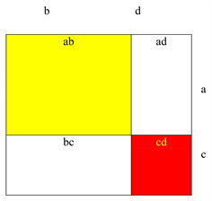
Theorem 1: Let A = ab, B = cd, C = ef, … be a rectangles then

$A+B=\left(a+c\right)\left(b+d\right)-\left(ad+bc\right)$. (1)

Proof: Let A = ab and B = cd then

$A+B=\left(a+c\right)\left(b+d\right)-\left(ad+bc\right)=ab+ad+bc+cd-ad-bc=ab+cd$ ■

Addition of two 3-dimensional cubes

Theorem 2: Let A = xyz and B = abc be a cubes then

$A+B=xyz+abc=\left(x+a\right)\left(y+b\right)\left(z+c\right)-\left(ayz+bxz+cxy+abz+bcx+cay\right)$ (2)

Proof: Let A = xyz and B = abc then

$\begin{array}{c}A+B=\left(x+a\right)\left(y+b\right)\left(z+c\right)-\left(ayz+bxz+cxy+abz+bcx+cay\right)\\ =xyz+ayz+bxz+cxy+abz+bcx+cay+abc\\ -\left(ayz+bxz+cxy+abz+bcx+cay\right)\\ =xyz+abc\end{array}$ ■

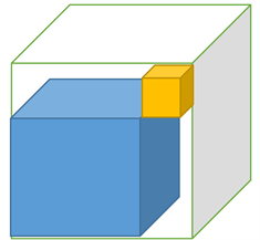
Definition 1: If two “n” cubes added, other than the sum of correspondence coordinates volume would be called as subtracting volumes. Which would be known as subtracting elements.

Theorem 3: Let $A=a_1{a}_2{a}_3\cdots a_n$ ; $B=b_1{b}_2{b}_3\cdots b_n$ ; $K=k_1{k}_2{k}_3\cdots k_n$ ; be n-dimensional cubes then the subtracting elements of $A+B+C+\cdots +K$ is

$K\left(K^{n-1}-1\right)=K^n-K$, (3)

where K is a number of n-dimensional cubes.

i.e. No. of $\left(a_1{b}_2{c}_3\cdots k_n+b_1{a}_2{c}_3\cdots k_n+c_1{b}_2{a}_3\cdots k_n+\cdots \right)$ is $K\left(K^{n-1}-1\right)$.

i.e. No. of subtracting elements is $K\left(K^{n-1}-1\right)$.

Ex 1:

1) Let A be the 5 × 6 sized rectangle and B be the 11 × 3 sized rectangle then area of A + B = (5 + 11)(6 + 3) − (15 + 66) = 16 × 9 − 81 = 144 − 81 = 63 = 30 + 33, where 30 is area of A and 33 is area of B. and the subtracting element (yellow colored) of A + B = 2. Where n = 2 and K = 2 then 2(2 − 1) = 2.

2) Let A = 7 × 8 sized rectangle, B = 19 × 7 sized rectangle, C = 23 × 2 sized rectangle then area of A + B + C = (7 + 19 + 23)(8 + 7 + 2) − (49 + 14 +152 + 38 + 184 + 161) = 49 × 17 – 598 = 235 = 56 + 133 + 46, where 30 is area of A, 33 is area of B 33 is area of C. And the subtracting element (yellow colored) of A + B + C = 6. In formula n = 2 and K = 3 then 3(3 − 1) = 3(2) = 6.

3) Let A = 5 × 6 × 7 sized cube and B = 11 × 3 × 8 sized cube then volume of A + B = (5 + 11)(6 + 3)(7 + 8) – (120 + 528 + 231 + 462 + 105 + 240) = 16 × 9 × 15 – 1617 = 2160 – 1686 = 474 = 210 + 264, where 210 is volume of A and 264 is volume of B. and the subtracting element (yellow colored) of A + B = 474. In formula n = 3 and K = 2 then 2(2³⁻¹ − 1) = 2(4 − 1) = 2(3) = 6.

4) Let A = abc, B = def and C = ghi sized cubes then volume of A + B + C = (a + d + g)(b + e + h)(c + f + i) – (abf + abi + aec + aef + aei + ahc + ahf + ahi + dbc + dbf + dbi + dec + dei + dhc + dhf + dhi + gbc + gbf + gbi + gec + gef + gei + ghc + ghf) = abc + def + ghi, where abc is volume of A, def is volume of B and ghi is volume of C. And the subtracting element (yellow colored) of A + B + C = 24. In formula n = 3 and K = 3 then 3(3³⁻¹ − 1) = 3(9 − 1) = 3(8) = 24.

Fact 1: How multiplication of matrices accepted by mathematicians? As far we know, matrix multiplications accepted by its determinant multiplication. Like that I am introducing some works by its determinants.

Addition of matrices

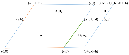
Addition of 2-dimensional matrix

Theorem 4: Let $A=\left(\begin{array}{cc}{a}_{11}& a_{12}\\ a_{21}& a_{22}\end{array}\right)$, $B=\left(\begin{array}{cc}{b}_{11}& b_{12}\\ b_{21}& b_{22}\end{array}\right)$, $C=\left(\begin{array}{cc}{c}_{11}& c_{12}\\ c_{21}& c_{22}\end{array}\right)$, $\cdots$ be a matrices then

$\left|A\right|+\left|B\right|=\left|A+B\right|-\left(\left|A_1{B}_2\right|+\left|B_1{A}_2\right|\right)$ (4)

where $\left|A_1{B}_2\right|=\left|\begin{array}{cc}{a}_{11}& a_{12}\\ b_{21}& b_{22}\end{array}\right|$ and $\left|B_1{A}_2\right|=\left|\begin{array}{cc}{b}_{11}& b_{12}\\ a_{21}& a_{22}\end{array}\right|$

$\left|A\right|+\left|B\right|+\left|C\right|=\left|A+B+C\right|-\left(\left|A_1{B}_2\right|+\left|A_1{C}_2\right|+\left|B_1{A}_2\right|+\left|B_1{C}_2\right|+\left|C_1{A}_2\right|+\left|C_1{B}_2\right|\right)$ (5)

…

$\begin{array}{l}\left|A\right|+\left|B\right|+\left|C\right|+\cdots +\left|N\right|\\ =\left|A+B+C+\cdots +N\right|-\left(\left|A_1{B}_2\right|+\left|A_1{C}_2\right|+\cdots +\left|A_1{N}_2\right|+\left|B_1{A}_2\right|+\left|B_1{C}_2\right|+\cdots \right)\end{array}$ (6)

Corollary 1: The number of subtracting matrices of two dimensional matrix addition is $k\left(k-\text{1}\right)$.

i.e. number of

$\left(\left|A_1{B}_2\right|+\left|A_1{C}_2\right|+\cdots +\left|A_1{N}_2\right|+\left|B_1{A}_2\right|+\left|B_1{C}_2\right|+\cdots \right)=k\left(k-1\right)$, (7)

where k is a number of matrices.

Addition of 3-dimensional matrix

Theorem 5: Let $A=\left(\begin{array}{ccc}{a}_{11}& a_{12}& a_{13}\\ a_{21}& a_{22}& a_{23}\\ a_{31}& a_{32}& a_{33}\end{array}\right)$, $B=\left(\begin{array}{ccc}{b}_{11}& b_{12}& b_{13}\\ b_{21}& b_{22}& b_{23}\\ b_{31}& b_{32}& b_{33}\end{array}\right)$, $C=\left(\begin{array}{ccc}{c}_{11}& c_{12}& c_{13}\\ c_{21}& c_{22}& c_{23}\\ c_{31}& c_{32}& c_{33}\end{array}\right)$, $\cdots$ be a matrices then

$\begin{array}{l}\left|A\right|+\left|B\right|\\ =\left|A+B\right|-\left(\left|A_1{B}_2{B}_3\right|+\left|B_1{A}_2{B}_3\right|+\left|B_1{B}_2{A}_3\right|+\left|A_1{A}_2{B}_3\right|+\left|B_1{A}_2{A}_3\right|+\left|A_1{B}_2{A}_3\right|\right)\end{array}$ (8)

where

$\left|A_1{B}_2{B}_3\right|=\left(\begin{array}{ccc}{a}_{11}& a_{12}& a_{13}\\ b_{21}& b_{22}& b_{23}\\ b_{31}& b_{32}& b_{33}\end{array}\right)$ ; $\left|B_1{A}_2{B}_3\right|=\left(\begin{array}{ccc}{b}_{11}& b_{12}& b_{13}\\ a_{21}& a_{22}& a_{23}\\ b_{31}& b_{32}& b_{33}\end{array}\right)$ ; $\left|B_1{B}_2{A}_3\right|=\left(\begin{array}{ccc}{b}_{11}& b_{12}& b_{13}\\ b_{21}& b_{22}& b_{23}\\ a_{31}& a_{32}& a_{33}\end{array}\right)$ ;

$\left|A_1{A}_2{B}_3\right|=\left(\begin{array}{ccc}{a}_{11}& a_{12}& a_{13}\\ a_{21}& a_{22}& a_{23}\\ b_{31}& b_{32}& b_{33}\end{array}\right)$ ; $\left|B_1{A}_2{A}_3\right|=\left(\begin{array}{ccc}{b}_{11}& b_{12}& b_{13}\\ a_{21}& a_{22}& a_{23}\\ a_{31}& a_{32}& a_{33}\end{array}\right)$ ; $\left|A_1{B}_2{A}_3\right|=\left(\begin{array}{ccc}{a}_{11}& a_{12}& a_{13}\\ b_{21}& b_{22}& b_{23}\\ a_{31}& a_{32}& a_{33}\end{array}\right)$ ;

$\begin{array}{l}\left|A\right|+\left|B\right|+\left|C\right|\\ =\left|A+B+C\right|-\left(\left|A_1{B}_2{C}_3\right|+\left|B_1{A}_2{C}_3\right|+\left|C_1{B}_2{A}_3\right|+\left|A_1{C}_2{B}_3\right|+\cdots +|\cdots |\right)\end{array}$ (9)

…

$\begin{array}{l}\left|A\right|+\left|B\right|+\left|C\right|+\cdots +\left|K\right|\\ =\left|A+B+C+\cdots +K\right|-\left(\left|A_1{B}_2{C}_3\right|+\left|B_1{A}_2{C}_3\right|+\left|C_1{B}_2{A}_3\right|+\cdots +\left|C_1{B}_2{K}_3\right|+\cdots \right)\end{array}$ (10)

Corollary 2: The number of subtracting matrices of 3-dimensional matrix addition is $k\left(k^2-1\right)$.

i.e. number of

$\left|A_1{B}_2{C}_3\right|+\left|B_1{A}_2{C}_3\right|+\left|C_1{B}_2{A}_3\right|+\cdots +\left|C_1{B}_2{N}_3\right|+\cdots =k\left(k^2-1\right)$, (11)

where k is a number of matrices.

Theorem 6: The number of subtracting matrices of n-dimensional matrix addition is $K\left(K^{n-1}-1\right)$.

i.e. number of

$\left|A_1{B}_2{C}_3\cdots K_n\right|+\left|B_1{A}_2{C}_3\cdots K_n\right|+\left|C_1{A}_2{B}_3\cdots K_n\right|+\cdots =K\left(K^{n-1}-1\right),$ (12)

where k is a number of matrices.

Ex 2:

1) Let $A=\left(\begin{array}{cc}5& 8\\ -3& 12\end{array}\right)$, $B=\left(\begin{array}{cc}7& 4\\ 6& 3\end{array}\right)$, be a matrices then $A+B=\left(\begin{array}{cc}12& 12\\ 3& 15\end{array}\right)$.

$\left|A\right|=84$ ; $\left|B\right|=-3$ ; $\left|A+B\right|=144$ ;

$A_1{B}_2=\left(\begin{array}{cc}5& 8\\ 6& 3\end{array}\right)$, $B_1{A}_2=\left(\begin{array}{cc}7& 4\\ -3& 12\end{array}\right)$ now, $\left|A_1{B}_2\right|=-33$ and $\left|B_1{A}_2\right|=96$

$\left|A\right|+\left|B\right|=\left|A+B\right|-\left[\left|A_1{B}_2\right|+\left|B_1{A}_2\right|\right]=144-\left[-33+96\right]=144-63=81$

No. of subtracting matrices = 2. ■

2) Let $A=\left(\begin{array}{ccc}-6& 9& -1\\ 8& -7& -1\\ -5& 2& -5\end{array}\right)$, $B=\left(\begin{array}{ccc}7& 2& 0\\ -2& -4& 7\\ -4& 0& 4\end{array}\right)$ be a matrices then $A+B=\left(\begin{array}{ccc}1& 11& -1\\ 6& -11& 6\\ -9& 2& -1\end{array}\right)$.

$\left|A\right|=202$ ; $\left|B\right|=-152$ ; and $\left|A+B\right|=-442$ ;

$B_1{A}_2{A}_3=\left(\begin{array}{ccc}7& 2& 0\\ 8& -7& -1\\ -5& 2& -5\end{array}\right)$, $A_1{B}_2{A}_3=\left(\begin{array}{ccc}-6& 9& -1\\ -2& -4& 7\\ -5& 2& -5\end{array}\right)$, $A_1{A}_2{B}_3=\left(\begin{array}{ccc}-6& 9& -1\\ 8& -7& -1\\ -4& 0& 4\end{array}\right)$,

$A_1{B}_2{B}_3=\left(\begin{array}{ccc}-6& 9& -1\\ -2& -4& 7\\ -4& 0& 4\end{array}\right)$, $B_1{A}_2{B}_3=\left(\begin{array}{ccc}7& 2& 0\\ 8& -7& -1\\ -4& 0& 4\end{array}\right)$, $B_1{B}_2{A}_3=\left(\begin{array}{ccc}7& 2& 0\\ -2& -4& 7\\ -5& 2& -5\end{array}\right)$

$\left|B_1{A}_2{A}_3\right|=349$, $\left|A_1{B}_2{A}_3\right|=-417$, $\left|A_1{A}_2{B}_3\right|=-56$, $\left|A_1{B}_2{B}_3\right|=-68$,

$\left|B_1{A}_2{B}_3\right|=-252$, $\left|B_1{B}_2{A}_3\right|=-48$ ;

$\begin{array}{l}\left|A\right|+\left|B\right|\\ =\left|A+B\right|-\left[\left|B_1{A}_2{A}_3\right|+\left|A_1{B}_2{A}_3\right|+\left|A_1{A}_2{B}_3\right|+\left|A_1{B}_2{B}_3\right|+\left|B_1{A}_2{B}_3\right|+\left|B_1{B}_2{A}_3\right|\right]\end{array}$

$\begin{array}{c}\left|A\right|+\left|B\right|=-442-\left[349-417-56-68-252-48\right]\\ =-442-\left[-492\right]=-442+492=50\end{array}$

No. of subtracting matrices = 6. ■

Subtraction of matrices

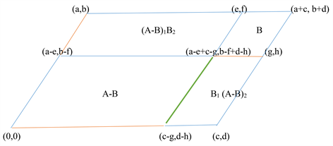
Theorem 8: Let A, B be a 2-dimensional matrices then

$\left|A\right|-\left|B\right|=\left|A-B\right|+\left|{\left(A-B\right)}_1{B}_2\right|+\left|B_1{\left(A-B\right)}_2\right|$, (13)

where $\left|{\left(A-B\right)}_1{B}_2\right|=\left|\begin{array}{cc}{a}_{11}-b_{11}& a_{12}-b_{12}\\ b_{21}& b_{22}\end{array}\right|$ and $\left|B_1{\left(A-B\right)}_2\right|=\left|\begin{array}{cc}{b}_{11}& b_{12}\\ a_{21}-b_{21}& a_{22}-b_{22}\end{array}\right|$.

Corollary 3: The number of adding matrices of two dimensional matrix subtraction is $k\left(k-1\right)$.

i.e. number of

$\begin{array}{l}\left(\left|{\left(A-B\right)}_1{B}_2\right|+\left|{\left(A-B\right)}_1{C}_2\right|+\cdots +\left|{\left(A-B\right)}_1{N}_2\right|+\left|B_1{\left(A-B\right)}_2\right|+\cdots \right)\\ =k\left(k-1\right)\end{array}$, (14)

where k is a number of matrices

Theorem 9: Let A, B be a 3-dimensional matrices then

$\begin{array}{c}\left|A\right|-\left|B\right|=\left|A-B\right|+\left|{\left(A-B\right)}_1{B}_2{B}_3\right|+\left|B_1{\left(A-B\right)}_2{B}_3\right|\\ +\left|B_1{B}_2{\left(A-B\right)}_3\right|+\left|{\left(A-B\right)}_1{\left(A-B\right)}_2{B}_3\right|\\ +\left|{\left(A-B\right)}_1{B}_2{\left(A-B\right)}_3\right|+\left|B_1{\left(A-B\right)}_2{\left(A-B\right)}_3\right|\end{array}$ (15)

Corollary 4: The number of adding matrices of 3-dimensional matrix subtraction is $k\left(k^2-1\right)$.

i.e. number of

$\left|{\left(A-B\right)}_1{B}_2{C}_3\right|+\left|B_1{\left(A-B\right)}_2{C}_3\right|+\left|C_1{B}_2{\left(A-B\right)}_3\right|+\cdots =k\left(k^2-1\right)$, (16)

where k is a number of matrices.

Theorem 10: The number of adding matrices of n-dimensional matrix subtraction is

$K\left(K^{n-1}-1\right)$. (17)

i.e. number of

$\begin{array}{l}\left|{\left(A-B\right)}_1{B}_2{C}_3\cdots K_n\right|+\left|B_1{\left(A-B\right)}_2{C}_3\cdots K_n\right|+\left|C_1{\left(A-B\right)}_2{B}_3\cdots K_n\right|+\cdots \\ =K\left(K^{n-1}-1\right),\end{array}$,

where K is a number of matrices.

Ex 3:

1) Let $A=\left(\begin{array}{cc}5& 8\\ -3& 12\end{array}\right)$, $B=\left(\begin{array}{cc}7& 4\\ 6& 3\end{array}\right)$, be a matrices then $A-B=\left(\begin{array}{cc}-2& 4\\ -9& 9\end{array}\right)$.

$\left|A\right|=84$ ; $\left|B\right|=-3$ ; $\left|A-B\right|=18$ ;

${\left(A-B\right)}_1{B}_2=\left(\begin{array}{cc}-2& 4\\ 6& 3\end{array}\right)$, $B_1{A}_2=\left(\begin{array}{cc}7& 4\\ -9& 9\end{array}\right)$ now, $\left|{\left(A-B\right)}_1{B}_2\right|=-30$ and $\left|B_1{\left(A-B\right)}_2\right|=99$

$\left|A\right|-\left|B\right|=\left|A-B\right|+\left|{\left(A-B\right)}_1{B}_2\right|+\left|B_1{\left(B-A\right)}_2\right|=18-30+99=117-30=87$.

No. of adding matrices = 2.■

2) Let $A=\left(\begin{array}{ccc}-6& 9& -1\\ 8& -7& -1\\ -5& 2& -5\end{array}\right)$, $B=\left(\begin{array}{ccc}7& 2& 0\\ -2& -4& 7\\ -4& 0& 4\end{array}\right)$ be a matrices then $A-B=\left(\begin{array}{ccc}-13& 7& -1\\ 10& -3& -8\\ -1& 2& -9\end{array}\right)$

$\left|A\right|=202$ ; $\left|B\right|=-152$ ; and $\left|A-B\right|=110$ ;

${\left(A-B\right)}_1{\left(A-B\right)}_2{B}_3=\left(\begin{array}{ccc}-13& 7& -1\\ 10& -3& -8\\ -4& 0& 4\end{array}\right)$, ${\left(A-B\right)}_1{B}_2{\left(A-B\right)}_3=\left(\begin{array}{ccc}-13& 7& -1\\ -2& -4& 7\\ -1& 2& -9\end{array}\right)$,

$B_1{\left(A-B\right)}_2{\left(A-B\right)}_3=\left(\begin{array}{ccc}7& 2& 0\\ 10& -3& -8\\ -1& 2& -9\end{array}\right)$, $B_1{B}_2{\left(A-B\right)}_3=\left(\begin{array}{ccc}7& 2& 0\\ -2& -4& 7\\ -1& 2& -9\end{array}\right)$,

$B_1{\left(A-B\right)}_2{B}_3=\left(\begin{array}{ccc}7& 2& 0\\ 10& -3& -8\\ -4& 0& 4\end{array}\right)$, ${\left(A-B\right)}_1{B}_2{B}_3=\left(\begin{array}{ccc}-13& 7& -1\\ -2& -4& 7\\ -4& 0& 4\end{array}\right)$

$\left|{\left(A-B\right)}_1{\left(A-B\right)}_2{B}_3\right|=112$, $\left|{\left(A-B\right)}_1{B}_2{\left(A-B\right)}_3\right|=-453$,

$\left|B_1{\left(A-B\right)}_2{\left(A-B\right)}_3\right|=497$,

$\left|B_1{B}_2{\left(A-B\right)}_3\right|=104$, $\left|B_1{\left(A-B\right)}_2{B}_3\right|=-100$, $\left|{\left(A-B\right)}_1{B}_2{B}_3\right|=84$ ;

$\begin{array}{c}\left|A\right|-\left|B\right|=\left|A-B\right|+\left|{\left(A-B\right)}_1{\left(A-B\right)}_2{B}_3\right|+\left|{\left(A-B\right)}_1{B}_2{\left(A-B\right)}_3\right|\\ +\left|B_1{\left(A-B\right)}_2{\left(A-B\right)}_3\right|+\left|B_1{B}_2{\left(A-B\right)}_3\right|\\ +\left|B_1{\left(A-B\right)}_2{B}_3\right|+\left|{\left(A-B\right)}_1{B}_2{B}_3\right|\end{array}$

$\left|A\right|-\left|B\right|=110+112-453+497+104-100+84=354$

No. of adding matrices = 6. ■

Division of fractions

$\frac{a}{b}÷\frac{c}{d}=\frac{e}{f}$, here we get quotient only not remainder.

If we piece an object by certain size of small pieces, we may get some pieces smaller than small pieces. These tiny pieces are called remainder of object and number of small pieces are called quotient of object.

Let us consider s as object, p as certain size of small pieces, q as number of p and r as reminded tiny pieces. Then for division formula we can say,

$s=pq+r$,

where q is quotient and r is remainder.

But in fractions,

$\frac{a}{b}÷\frac{c}{d}=\frac{e}{f}$,

here we get quotient only, not remainder!

Is it possible? Or is it right way to find quotient and remainder?

We do just a small modification in above formula.

Now

$\frac{a}{b}÷\frac{c}{d}=\frac{e}{f}=k\frac{s}{f}=k\left(\frac{c}{d}\right)+\frac{s}{f}\left(\frac{c}{d}\right)$, (18)

where k is quotient of above division and $\frac{s}{f}\left(\frac{c}{d}\right)=r$ is a remainder of above division.

Ex:

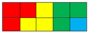
1) Let $\frac{5}{2}÷\frac{3}{4}$ then $\frac{5}{2}÷\frac{3}{4}=\frac{10}{3}$ ;

$\Rightarrow \frac{10}{3}=3\frac{1}{3}$ ;

$\frac{5}{2}=3\frac{1}{3}\left(\frac{3}{4}\right)=3\left(\frac{3}{4}\right)+\frac{1}{3}\left(\frac{3}{4}\right)=3\left(\frac{3}{4}\right)+\frac{1}{4}$ ; 3 is a quotient and $\frac{1}{4}$ is remainder.

$\Rightarrow 3\left(\frac{3}{4}\right)+\frac{1}{4}=\frac{9}{4}+\frac{1}{4}=\frac{10}{4}$

So we get

$\Rightarrow \frac{5}{2}\equiv \frac{10}{4}$.

In picture:

Four small squares construct one unit square, $\frac{5}{2}$ means two unit square + one half unit square. $\frac{3}{4}$ Means three small squares. Now, let us fill squares by colors.

2) $\frac{3}{4}÷\frac{5}{2}$ then $\frac{3}{4}÷\frac{5}{2}=\frac{3}{10}$ ; where $\frac{3}{4}<\frac{5}{2}$, so we can say $\frac{3}{10}\left(\frac{5}{2}\right)=0\left(\frac{5}{2}\right)+\frac{3}{10}\left(\frac{5}{2}\right)=0\left(\frac{5}{2}\right)+\frac{15}{20}=\frac{3}{4}$ ; 0 is a quotient and $\frac{3}{4}$ is remainder.

Facts

1) $\left|A\pm B\right|\ne \left|A\right|\pm \left|B\right|$ but now, we could find $\left|A\pm B\right|=\left|A\right|\pm \left|B\right|$

2) $\left|AB\right|=\left|A\right|\left|B\right|$

3) $\left|k{B}_n\right|=k^n\left|B_n\right|$

4) $A=qB+r$

Let A and B be any two matrices with same dimensional then can we write $A=qB+r$ ? Where q is a quotient matrix (number of B in A) and r is remainder matrix.

Definition 2 (matrix division):

Let A be a dividend matrix and B be a divisor matrix then $A=qB+r$, where q is a quotient matrix of A and r is a remainder matrix of A.

Finding q and r:

Let us divide determinant of A matrix by determinant of B matrix then we get k.d₁d₂d₃d₄ …. where k is a numeral part which is the determinant of quotient q matrix and d₁d₂d₃d₄ …. is a decimal part which is remainder multiplier matrix of divisor B.

We know $\left|AB\right|=\left|A\right|\left|B\right|$. So we can write

$\frac{A}{B}=A{B}^{-1}\Rightarrow \left|\frac{A}{B}\right|=\left|A{B}^{-1}\right|=\left|A\right|\left|B^{-1}\right|=k.d_1{d}_2{d}_3{d}_4\cdots =\frac{\left|A\right|}{\left|B\right|}$

Using formula (18), we get

i.e. $\left[A\right]\equiv \left[k^{\frac{1}{n}}\right]\left[B\right]+\left[{\left(0.d_1{d}_2{d}_3\cdots \right)}^{\frac{1}{n}}\right]\left[B\right]\equiv \left[k^{\frac{1}{n}}\right]\left[B\right]+\left[r\right]$ (19)

where $\left[k^{\frac{1}{n}}\right]$ is a quotient and $\left[r\right]$ is a remainder.

Steps for matrix division

1) Let A be a dividend matrix and B be a divisor matrix.

2) Find determinant of A and B matrix.

3) If $\left|A\right|\ne 0$ and $\left|B\right|\ne 0$ then only proceed next step.

4) Find $\frac{\left|A\right|}{\left|B\right|}$.

5) If $\frac{\left|A\right|}{\left|B\right|}=k.d_1{d}_2{d}_3\cdots$ then separate integer part for quotient and decimal part for remainder.

6) Find the diagonal quotient matrix which should give determinant value equal to k and also find the diagonal remainder multiplier matrix which should give determinant value equal to d₁d₂d₃ …

7) Now write $\left[A\right]\equiv \left[k^{\frac{1}{n}}\right]\left[B\right]+\left[{\left(0.d_1{d}_2{d}_3\cdots \right)}^{\frac{1}{n}}\right]\left[B\right]\equiv \left[k^{\frac{1}{n}}\right]\left[B\right]+\left[r\right]$ where $\left[k^{\frac{1}{n}}\right]$ is a quotient matrix and $\left[r\right]$ is a remainder matrix.

8) Check the compatibility by finding determinant for A and its equivalent. i.e. $\left|A\right|=\left|k^{\frac{1}{n}}\right|\left|B\right|+\left|r\right|$.

Ex 4:

1) Let $A=\left(\begin{array}{cc}1& 0\\ 0& 17\end{array}\right)$ and $B=\left(\begin{array}{cc}2& 1\\ 4& 3\end{array}\right)$ then $\left|A\right|=17$ and $\left|B\right|=2$.

Now $B^{-1}=\frac{1}{2}\left(\begin{array}{cc}3& -1\\ -4& 2\end{array}\right)=\left(\begin{array}{cc}\frac{3}{2}& \frac{-1}{2}\\ -2& 1\end{array}\right)$, so $\left|B^{-1}\right|=\frac{1}{2}$ ;

$A{B}^{-1}=\left(\begin{array}{cc}1& 0\\ 0& 17\end{array}\right)\left(\begin{array}{cc}\frac{3}{2}& \frac{-1}{2}\\ -2& 1\end{array}\right)=\left(\begin{array}{cc}\frac{3}{2}& \frac{-1}{2}\\ -34& 17\end{array}\right)$

$\left|A{B}^{-1}\right|=\left|\begin{array}{cc}\frac{3}{2}& \frac{-1}{2}\\ -34& 17\end{array}\right|=\frac{51}{2}-17=\frac{51-34}{2}=\frac{17}{2}=8.5=8\frac{1}{2}$

Hence, $\left|\frac{A}{B}\right|=\left|A\right|\left|B^{-1}\right|=17\times \frac{1}{2}=8.5$

Like divisions of fractions we can write, $A=8B+\frac{1}{2}B$

In matrix term we write above sum as $A\equiv \left[2\sqrt{2}\right]B+\left[\frac{1}{\sqrt{2}}\right]B$

Since $\left[8^{\frac{1}{2}}\right]=\left[2\sqrt{2}\right]$ and $\left[{\left(\frac{1}{2}\right)}^{\frac{1}{2}}\right]=\left[\frac{1}{\sqrt{2}}\right]$

$\left(\begin{array}{cc}1& 0\\ 0& 17\end{array}\right)\equiv \left(\begin{array}{cc}2\sqrt{2}& 0\\ 0& 2\sqrt{2}\end{array}\right)\left(\begin{array}{cc}2& 1\\ 4& 3\end{array}\right)+\left(\begin{array}{cc}\frac{1}{\sqrt{2}}& 0\\ 0& \frac{1}{\sqrt{2}}\end{array}\right)\left(\begin{array}{cc}2& 1\\ 4& 3\end{array}\right)$

$\left(\begin{array}{cc}1& 0\\ 0& 17\end{array}\right)\equiv \left(\begin{array}{cc}2\sqrt{2}& 0\\ 0& 2\sqrt{2}\end{array}\right)\left(\begin{array}{cc}2& 1\\ 4& 3\end{array}\right)+\left(\begin{array}{cc}\frac{2}{\sqrt{2}}& \frac{1}{\sqrt{2}}\\ \frac{4}{\sqrt{2}}& \frac{3}{\sqrt{2}}\end{array}\right)$, where $\left(\begin{array}{cc}2\sqrt{2}& 0\\ 0& 2\sqrt{2}\end{array}\right)$ is quotient and $\left(\begin{array}{cc}\frac{2}{\sqrt{2}}& \frac{1}{\sqrt{2}}\\ \frac{4}{\sqrt{2}}& \frac{3}{\sqrt{2}}\end{array}\right)$ is remainder.

$LHS=\left|\begin{array}{cc}1& 0\\ 0& 17\end{array}\right|=17$

$\left|\begin{array}{cc}2\sqrt{2}& 0\\ 0& 2\sqrt{2}\end{array}\right|\left|\begin{array}{cc}2& 1\\ 4& 3\end{array}\right|+\left|\begin{array}{cc}\frac{2}{\sqrt{2}}& \frac{1}{\sqrt{2}}\\ \frac{4}{\sqrt{2}}& \frac{3}{\sqrt{2}}\end{array}\right|=8\times 2+1=17=RHS$.

2) Let $A=\left(\begin{array}{cc}2& 0\\ 0& 15\end{array}\right)$ and $B=\left(\begin{array}{cc}2& 0\\ 0& 3\end{array}\right)$ then $\left|A\right|=30$ and $\left|B\right|=6$.

Now $B^{-1}=\frac{1}{6}\left(\begin{array}{cc}3& 0\\ 0& 2\end{array}\right)=\left(\begin{array}{cc}\frac{3}{6}& 0\\ 0& \frac{2}{6}\end{array}\right)$, so $\left|B^{-1}\right|=\frac{1}{6}$ ;

Hence, $\left|\frac{A}{B}\right|=\left|A\right|\left|B^{-1}\right|=30\times \frac{1}{6}=5$

Like divisions of fractions we can write,

$A=5B+0B$

In matrix term we write above sum as $A=\left[\sqrt{5}\right]B+\left[0\right]B$

$\left(\begin{array}{cc}2& 0\\ 0& 15\end{array}\right)\equiv \left(\begin{array}{cc}\sqrt{5}& 0\\ 0& \sqrt{5}\end{array}\right)\left(\begin{array}{cc}2& 0\\ 0& 3\end{array}\right)+\left(\begin{array}{cc}0& 0\\ 0& 0\end{array}\right)\equiv \left(\begin{array}{cc}2\sqrt{5}& 0\\ 0& 3\sqrt{5}\end{array}\right)+\left(\begin{array}{cc}0& 0\\ 0& 0\end{array}\right)$, where $\left(\begin{array}{cc}\sqrt{5}& 0\\ 0& \sqrt{5}\end{array}\right)$ is quotient and $\left(\begin{array}{cc}0& 0\\ 0& 0\end{array}\right)$ is remainder.

$LHS=\left|\begin{array}{cc}2& 0\\ 0& 15\end{array}\right|=30$

$\left|\begin{array}{cc}\sqrt{5}& 0\\ 0& \sqrt{5}\end{array}\right|\left|\begin{array}{cc}2& 0\\ 0& 3\end{array}\right|=5\times 6=30=RHS$.

3) Let $A=\left(\begin{array}{cc}2& 1\\ 4& 3\end{array}\right)$ and $B=\left(\begin{array}{cc}3& 5\\ 1& 5\end{array}\right)$ then $\left|A\right|=2$ and $\left|B\right|=10$.

Now $B^{-1}=\frac{1}{10}\left(\begin{array}{cc}5& -5\\ -1& 3\end{array}\right)=\left(\begin{array}{cc}\frac{5}{10}& \frac{-5}{10}\\ \frac{-1}{10}& \frac{3}{10}\end{array}\right)$, so $\left|B^{-1}\right|=\frac{1}{10}$ ;

Hence, $\left|\frac{A}{B}\right|=\left|A\right|\left|B^{-1}\right|=2\times \frac{1}{10}=\frac{2}{10}=\frac{1}{5}$

Like divisions of fractions we can write,

$A=0B+\frac{1}{5}B=\frac{1}{5}B$

In matrix term we write above sum as $A=\left[0\right]B+\left[\frac{1}{\sqrt{5}}\right]B$

$\left(\begin{array}{cc}2& 1\\ 4& 3\end{array}\right)\equiv \left(\begin{array}{cc}0& 0\\ 0& 0\end{array}\right)\left(\begin{array}{cc}3& 5\\ 1& 5\end{array}\right)+\left(\begin{array}{cc}\frac{1}{\sqrt{5}}& 0\\ 0& \frac{1}{\sqrt{5}}\end{array}\right)\left(\begin{array}{cc}3& 5\\ 1& 5\end{array}\right)=\left(\begin{array}{cc}\frac{3}{\sqrt{5}}& \frac{5}{\sqrt{5}}\\ \frac{1}{\sqrt{5}}& \frac{5}{\sqrt{5}}\end{array}\right)$

$\left(\begin{array}{cc}2& 1\\ 4& 3\end{array}\right)\equiv \left(\begin{array}{cc}\frac{3}{\sqrt{5}}& \frac{5}{\sqrt{5}}\\ \frac{1}{\sqrt{5}}& \frac{5}{\sqrt{5}}\end{array}\right)$, where $\left(\begin{array}{cc}0& 0\\ 0& 0\end{array}\right)$ is quotient and $\left(\begin{array}{cc}\frac{3}{\sqrt{5}}& \frac{5}{\sqrt{5}}\\ \frac{1}{\sqrt{5}}& \frac{5}{\sqrt{5}}\end{array}\right)$ is remainder.

$LHS=\left|\begin{array}{cc}2& 1\\ 4& 3\end{array}\right|=2$

$\left|\begin{array}{cc}\frac{3}{\sqrt{5}}& \frac{5}{\sqrt{5}}\\ \frac{1}{\sqrt{5}}& \frac{5}{\sqrt{5}}\end{array}\right|=2=RHS$.

It is also true for B⁻¹A.

4) Let $A=\left(\begin{array}{cc}1& 0\\ 0& 17\end{array}\right)$ and $B=\left(\begin{array}{cc}2& 1\\ 4& 3\end{array}\right)$ then $\left|A\right|=17$ and $\left|B\right|=2$.

Now $B^{-1}=\frac{1}{2}\left(\begin{array}{cc}3& -1\\ -4& 2\end{array}\right)=\left(\begin{array}{cc}\frac{3}{2}& \frac{-1}{2}\\ -2& 1\end{array}\right)$, so $\left|B^{-1}\right|=\frac{1}{2}$ ;

$B^{-1}A=\left(\begin{array}{cc}\frac{3}{2}& \frac{-1}{2}\\ -2& 1\end{array}\right)\left(\begin{array}{cc}1& 0\\ 0& 17\end{array}\right)=\left(\begin{array}{cc}\frac{3}{2}& \frac{-17}{2}\\ -2& 17\end{array}\right)$

$\left|B^{-1}A\right|=\left|\begin{array}{cc}\frac{3}{2}& \frac{-17}{2}\\ -2& 17\end{array}\right|=\frac{51}{2}-17=\frac{51-34}{2}=\frac{17}{2}=8.5=8\frac{1}{2}$

Hence, $\left|\frac{A}{B}\right|=\left|B^{-1}\right|\left|A\right|=\frac{1}{2}\times 17=8.5$

Like divisions of fractions we can write, $A=B8+B\frac{1}{2}$

In matrix term we write above sum as $A\equiv B\left[2\sqrt{2}\right]+B\left[\frac{1}{\sqrt{2}}\right]$

Since $\left[8^{\frac{1}{2}}\right]=\left[2\sqrt{2}\right]$ and $\left[{\left(\frac{1}{2}\right)}^{\frac{1}{2}}\right]=\left[\frac{1}{\sqrt{2}}\right]$

$\left(\begin{array}{cc}1& 0\\ 0& 17\end{array}\right)\equiv \left(\begin{array}{cc}2& 1\\ 4& 3\end{array}\right)\left(\begin{array}{cc}2\sqrt{2}& 0\\ 0& 2\sqrt{2}\end{array}\right)+\left(\begin{array}{cc}2& 1\\ 4& 3\end{array}\right)\left(\begin{array}{cc}\frac{1}{\sqrt{2}}& 0\\ 0& \frac{1}{\sqrt{2}}\end{array}\right)$

$\left(\begin{array}{cc}1& 0\\ 0& 17\end{array}\right)\equiv \left(\begin{array}{cc}2& 1\\ 4& 3\end{array}\right)\left(\begin{array}{cc}2\sqrt{2}& 0\\ 0& 2\sqrt{2}\end{array}\right)+\left(\begin{array}{cc}\frac{2}{\sqrt{2}}& \frac{1}{\sqrt{2}}\\ \frac{4}{\sqrt{2}}& \frac{3}{\sqrt{2}}\end{array}\right)$ where $\left(\begin{array}{cc}2\sqrt{2}& 0\\ 0& 2\sqrt{2}\end{array}\right)$ is quotient and $\left(\begin{array}{cc}\frac{2}{\sqrt{2}}& \frac{1}{\sqrt{2}}\\ \frac{4}{\sqrt{2}}& \frac{3}{\sqrt{2}}\end{array}\right)$ is remainder.

Let we find a equivalence matrix for A matrix when A matrix divided by $\left(\begin{array}{cc}2& 1\\ 4& 3\end{array}\right)$

$A\equiv qB+r\equiv \left(\begin{array}{cc}4\sqrt{2}& 2\sqrt{2}\\ 8\sqrt{2}& 6\sqrt{2}\end{array}\right)+\left(\begin{array}{cc}\frac{2}{\sqrt{2}}& \frac{1}{\sqrt{2}}\\ \frac{4}{\sqrt{2}}& \frac{3}{\sqrt{2}}\end{array}\right)=\left(\begin{array}{cc}4\sqrt{2}+\frac{2}{\sqrt{2}}& 2\sqrt{2}+\frac{1}{\sqrt{2}}\\ 8\sqrt{2}+\frac{4}{\sqrt{2}}& 6\sqrt{2}+\frac{3}{\sqrt{2}}\end{array}\right)\equiv \left(\begin{array}{cc}\frac{10}{\sqrt{2}}& \frac{5}{\sqrt{2}}\\ \frac{20}{\sqrt{2}}& \frac{15}{\sqrt{2}}\end{array}\right)$

where $\left(\begin{array}{cc}\frac{10}{\sqrt{2}}& \frac{5}{\sqrt{2}}\\ \frac{20}{\sqrt{2}}& \frac{15}{\sqrt{2}}\end{array}\right)$ is a equivalence matrix of matrix A.

$\begin{array}{c}\left|qB\right|+\left|r\right|=\left|qB+r\right|-\left(\left|q{B}_1{r}_2\right|+\left|r_{1}q{B}_2\right|\right)\\ =\left|\begin{array}{cc}\frac{10}{\sqrt{2}}& \frac{5}{\sqrt{2}}\\ \frac{20}{\sqrt{2}}& \frac{15}{\sqrt{2}}\end{array}\right|-\left[\left|\begin{array}{cc}4\sqrt{2}& 2\sqrt{2}\\ \frac{4}{\sqrt{2}}& \frac{3}{\sqrt{2}}\end{array}\right|+\left|\begin{array}{cc}\frac{2}{\sqrt{2}}& \frac{1}{\sqrt{2}}\\ 8\sqrt{2}& 6\sqrt{2}\end{array}\right|\right]\\ =25-\left[4+4\right]=25-8=17\end{array}$

Hence $\left|A\right|=\left|qB\right|+\left|r\right|$, since $\left|A\right|=17$ ■

5) If $A=\left[\begin{array}{ccc}-9& -6& 6\\ 5& 2& 5\\ 5& 2& -7\end{array}\right]$ be a dividend matrix and $B=\left[\begin{array}{ccc}5& -3& -1\\ -6& 2& -7\\ -2& -2& -5\end{array}\right]$ be a divisor matrix then find the remainder matrix of $\frac{A}{B}$ ?

Solution:

Let $A=\left[\begin{array}{ccc}-9& -6& 6\\ 5& 2& 5\\ 5& 2& -7\end{array}\right]$ be a dividend matrix then $\left|A\right|=-144\ne 0$

And let $B=\left[\begin{array}{ccc}5& -3& -1\\ -6& 2& -7\\ -2& -2& -5\end{array}\right]$ be a divisor matrix then $\left|B\right|=-88\ne 0$

Now $\frac{\left|A\right|}{\left|B\right|}=\frac{-144}{-88}=1.6363$

Given matrices, A and B are 3 × 3 matrices. So the quotient diagonal matrix and remainder multiplier diagonal matrix should be 3 × 3 matrix.

Numeral part is 1, so quotient diagonal matrix would be $q=\left[\begin{array}{ccc}1& 0& 0\\ 0& 1& 0\\ 0& 0& 1\end{array}\right]$

$qB=\left[\begin{array}{ccc}1& 0& 0\\ 0& 1& 0\\ 0& 0& 1\end{array}\right]\left[\begin{array}{ccc}5& -3& -1\\ -6& 2& -7\\ -2& -2& -5\end{array}\right]$

Decimal part is 0.6363, remainder multiplier diagonal matrix would be $0.d_1{d}_2{d}_3\cdots =\left[\begin{array}{ccc}0.86& 0& 0\\ 0& 0.86& 0\\ 0& 0& 0.86\end{array}\right]$

Thus, remainder matrix

$r=\left[\begin{array}{ccc}0.86& 0& 0\\ 0& 0.86& 0\\ 0& 0& 0.86\end{array}\right]\left[\begin{array}{ccc}5& -3& -1\\ -6& 2& -7\\ -2& -2& -5\end{array}\right]=\left[\begin{array}{ccc}4.3& -2.58& -0.86\\ -5.16& 1.72& -6.02\\ -1.72& -1.72& -4.3\end{array}\right]$

From the above we get $\left|qB\right|=-88$ and $\left|r\right|=-55.97\cong -56$

$\Rightarrow \left|qB\right|+\left|r\right|=-88-56=-144=\left|A\right|$.

Let we find the equivalence matrix for matrix A

Equivalence matrix of A when divided by $B=\left[\begin{array}{ccc}5& -3& -1\\ -6& 2& -7\\ -2& -2& -5\end{array}\right]$

$\begin{array}{c}A=qB+r=\left[\begin{array}{ccc}5& -3& -1\\ -6& 2& -7\\ -2& -2& -5\end{array}\right]+\left[\begin{array}{ccc}4.3& -2.58& -0.86\\ -5.16& 1.72& -6.02\\ -1.72& -1.72& -4.3\end{array}\right]\\ =\left[\begin{array}{ccc}9.3& -5.58& -1.86\\ -11.16& 3.72& -13.02\\ -3.72& -3.72& -9.3\end{array}\right]\end{array}$

$\left|qB+r\right|=-566$

Using Equation (8),

$\left|qB\right|+\left|r\right|=\left|Q+r\right|-\left(\left|Q_1{r}_2{r}_3\right|+\left|r_1{Q}_2{r}_3\right|+\left|r_1{r}_2{Q}_3\right|+\left|Q_1{Q}_2{r}_3\right|+\left|r_1{Q}_2{Q}_3\right|+\left|Q_1{r}_2{Q}_3\right|\right)$

where Q is considered as qB matrix and r is a remainder matrix.

$S_1=\left[\begin{array}{ccc}4.3& -2.58& -0.86\\ -6& 2& -7\\ -2& -2& -5\end{array}\right]$ ; $S_2=\left[\begin{array}{ccc}5& -3& -1\\ -5.16& 1.72& -6.02\\ -2& -2& -5\end{array}\right]$ ;

$S_3=\left[\begin{array}{ccc}5& -3& -1\\ -6& 2& -7\\ -1.72& -1.72& -4.3\end{array}\right]$ ; $S_4=\left[\begin{array}{ccc}5& -3& -1\\ -5.16& 1.72& -6.02\\ -1.72& -1.72& -4.3\end{array}\right]$ ;

$S_5=\left[\begin{array}{ccc}4.3& -2.58& -0.86\\ -6& 2& -7\\ -1.72& -1.72& -4.3\end{array}\right]$ ; $S_6=\left[\begin{array}{ccc}4.3& -2.58& -0.86\\ -5.16& 1.72& -6.02\\ -2& -2& -5\end{array}\right]$ ;

where S₁ to S₆ are considered as subtracting matrices

$\left|S_1\right|=-75.7$ ;

$\left|S_2\right|=-75.7$ ;

$\left|S_3\right|=-75.7$ ;

$\left|S_4\right|=-65.1$ ;

$\left|S_5\right|=-65.1$ ;

$\left|S_6\right|=-65.1$ ;

Hence,

$\begin{array}{c}\left|qB\right|+\left|r\right|=-566.267-\left(-75.7-75.7-75.7-65.1-65.1-65.1\right)\\ =-566.267+422.4=-143.867\cong -144=\left|A\right|\end{array}$

■

Theorem 11: If $\frac{A}{B_L}=B\times q_{L}I+r_L$ and $\frac{A}{B_R}=q_{R}I\times B+r_R$ then equivalence matrix of $A\equiv qB+r$,

Proof: Let A be a dividend matrix and B be a divisor matrix then if we divide matrix A-volume by matrix B-volume from left to right we get

$\frac{A}{B_L}=B^{-1}A=B\times q_{L}I+r_L$ ;(20)

And if we divide matrix A-volume by matrix B-volume from right to left we get

$\frac{A}{B_R}=A{B}^{-1}=q_{R}I\times B+r_R$ ; (21)

$q_L,q_R,r_L$ and $r_R$ are diagonal matrices. In which $q_L,q_R$ has same elements and $r_L,r_R$ has same elements

So, we can claim $q_L=q_R$ and $r_L=r_R$ ;

Now,

$\frac{A}{B_L}=B^{-1}A\equiv B\times q_{L}I+r_L=q_{R}I\times B+r_R\equiv A{B}^{-1}=\frac{A}{B_R}$ (22)

So we concluded, $q_L=q_R=q$ and $r_L=r_R=r$

Hence, we can find equivalence matrix of

$A\equiv qB+r$. (23)

2. Conclusions

1) We can derive seven matrices from a given matrix.

2) Determinant of matrix addition has $K\left(K^{n-1}-1\right)$ subtracting matrices.

3) Determinant of matrix subtraction has $K\left(K^{n-1}-1\right)$ adding matrices.

4) Division of fractions is a good way of volumetric expressions.

5) We can divide matrix and we also can find remainder matrix.

6) If we add quotient matrix times of divisor matrix with remainder matrix, we may get equivalence matrix of dividend matrix.

7) Left division and right division give same equivalence matrix for dividend matrix.

Conflicts of Interest

The author declares no conflicts of interest regarding the publication of this paper.

References

[1]	Wikipedia. http://en.wikipedia.org/wiki/Matrix_
[2]	Lipschuts, S. and Lipson, M.L. (2011) Theory and Problems of Linear Algebra. 3rd Edition, Tata McGraw-Hill, India.
[3]	Rangasamy, B.P. (2019) Matrices—One Review. Advances in Linear Algebra & Matrix Theory, 9, 43-72. https://doi.org/10.4236/alamt.2019.93004
[4]	Rangasamy, B.P. (2020) One Approach to Matrix. International Journal of Innovative Studies in Sciences and Engineering Technology, 6, 38-45. https://ijisset.org/