The Global Attractors and Dimensions Estimation for the Higher-Order Nonlinear Kirchhoff-Type Equation with Strong Damping

Guoguang Lin, Yalan Yang

School of Mathematics and Statistics, Yunnan University, Kunming, China.

DOI: 10.4236/ijmnta.2020.94005                

Abstract

The initial boundary value problems for a class of high order Kirchhoff type equations with nonlinear strongly damped terms are considered. We establish the existence and uniqueness of the global solution of the problem by using prior estimates and Galerkin’s method under proper assumptions for the rigid term. Then the compact method is used to prove the existence of a compact family of global attractors in the solution semigroup generated by the problem. Finally, the Frechet differentiability of the operator semigroup and the decay of the volume element of linearization problem are proved, and the Hausdorff dimension and Fractal dimension of the family of global attractors are obtained.

Keywords

Nonlinear Higher-Order Kirchhoff Type Equation, The Priori Estimates, The Galerkin’s Method, The Global Attractors, Dimension Estimation

1. Introduction

The study of dynamical system is closely related to some important problems in natural science (such as turbulence in fluid mechanics, three-body problem in celestial mechanics, etc.), which attract a large number of natural scientists to study for a long time. However, the content of general research is limited to the case of finite dimension. With the development of science and technology, especially the rapid development of computer technology, it is already possible to learn more about the evolution and final state of infinite dimensional dynamical systems through computers. Since the 1980s, the infinite dimensional dynamical system has been studied in detail, such as the Russian mathematician O. A. Ladyzhenskoya ( [1] [2] [3] ), French mathematician R. Temam ( [4] [5] ), American mathematician G. Sell [6] and Guo Boling [7] who is an academician of the Chinese. They have made a deep research on a kind of infinite dimensional dynamical system generated by a class of nonlinear development equations with dissipative effects. Under certain conditions, it is proved that all these systems have a global attractor. Furthermore, the upper and lower bounds of the Hausdorff dimension and Fractal dimension of the global attractor are estimated. Many monographs have been published in this field, see ( [8] [9] [10] [11] ). Igor et al. [8] considered the long-time behavior of solutions to a damped wave equation with a critical source term and investigated the existence and various properties of global attractors. In [9] , Yang and Wang considered the longtime behavior of solution for the following Kirchhoff type equation with a strong dissipation:

$u_{tt}-M\left({\Vert \nabla u\Vert }^2\right)-\Delta u_t+h\left(u_t\right)+g\left(u\right)=f\left(x\right)\mathrm{.}$

They proved that the related continuous semigroup $S\left(t\right)$ possesses in the phase space with low regularity a global attractor that is connected. Kirchhoff type differential equations are a kind of classical problems in partial differential equations. In 1883, German physicist G. Kirchhoff [12] established the equation when he studied the vibration of strings.

$\rho h{u}_{tt}=\left\{p_0+\frac{Eh}{2L}{\displaystyle {\int }_0^L}{u}_x^2\text{d}x\right\}{u}_{xx}+f,0<x<L,t\ge 0.$

where $u=u\left(x\mathrm{,}t\right)$ is the lateral displacement under space coordinate x and time coordinate t, E the Young modulus, $\rho$ the mass density, h the cross-sectional area, L the length, p₀ the initial axial tension, f the external force. It corrects the classic D’alembert wave equation. Thus, the process of string vibration is described more precisely. This model has been widely used in non-newtonian fluid mechanics, astrophysics, image processing, plasma problems and elastic theory. Early research on the Kirchhoff type equations could be found in the literature ( [13] - [20] ).

Wu and Tsai [21] studied the initial boundary value problem of the following Kirchhoff-type beam equation

$u_{tt}+a{\Delta }^{2}u-M\left({\Vert Du\Vert }^2\right)\Delta u+g\left(u_t\right)=f\left(u\right)\mathrm{,}$

$u\left(x,0\right)=u_0\left(x\right),u_t\left(x,0\right)=u_1\left(x\right),$

$u\left(x,t\right)=0,\frac{\partial u}{\partial \upsilon }=0,x\in \partial \Omega ,t>0.$

They prove that the existence and uniqueness of the global solution and the decay estimation.

In the process of vibration and deformation of the vibration system, the characteristic that the amplitude of the vibration gradually decreases due to the inherent reasons of the system or the interaction with the outside world is called damping, and mathematically called dissipation.

Igor Chueshov [22] studied long-time dynamics of a class of quasilinear wave equations with a strong damping term

$u_{tt}-\sigma \left({\Vert Du\Vert }^2\right)\Delta u_t-\varphi \left({\Vert Du\Vert }^2\right)\Delta u+f\left(u\right)=h\left(x\right)\mathrm{,}$

$u\left(x\mathrm{,}t\right)=\mathrm{0,}x\in \partial \Omega \mathrm{,}$

$u\left(x\mathrm{,0}\right)=u_0\left(x\right)\mathrm{,}{u}_t\left(x\mathrm{,0}\right)=u_1\left(x\right)\mathrm{.}$

They proved the existence and uniqueness of the weak solutions and studied their properties for a wide class of nonlinearities which covers the case of possible degeneration (or even negativity) of the stiffness coefficient and the case of a supercritical source term. They also established the existence of a fractal exponential attractor and give conditions that guarantee the existence of a finite number of determining functionals.

Recently, Guoguang Lin, Zhuoxi Li [23] studied the initial boundary value problem for a class of high order Kirchhoff type equations with nonlinear non-local source term and strongly damped term

$u_{tt}+M\left({\Vert D^{m}u\Vert }^2\right){\left(-\Delta \right)}^{m}u+\beta {\left(-\Delta \right)}^m{u}_t+g\left(x\mathrm{,}u\right)=f\left(x\right)\mathrm{,}$

$u\left(x,t\right)=0,\frac{{\partial }^{i}u}{\partial {\upsilon }^i}=0,i=1,2,\cdots ,m-1,x\in \partial \Omega ,t>0,$

$u\left(x,0\right)=u_0\left(x\right),u_t\left(x,0\right)=u_1\left(x\right),x\in \Omega \subset R^n.$

where $m>1$ is a positive integer, $f\left(x\right)$ is an external force term, $g\left(x\mathrm{,}u\right)$ is a nonlinear non-local source term.

They proved that the existence of the family of global attractors and estimated their Hausdorff dimensions and Fractal dimensions.

In the present paper, we deal with the following the higher-order nonlinear Kirchhoff type problem involving a strong damping term

$u_{tt}+M\left({\Vert D^{m}u\Vert }_p^p\right){\left(-\Delta \right)}^{m}u+{\Delta }^{2m}u+\beta {\left(-\Delta \right)}^m{u}_t=g\left(x\right)\mathrm{,}$ (1)

$u\left(x,t\right)=0,\frac{{\partial }^{i}u}{\partial {\upsilon }^i}=0,i=1,2,\cdots ,2m-1,x\in \partial \Omega ,t>0,$ (2)

$u\left(x,0\right)=u_0\left(x\right),u_t\left(x,0\right)=u_1\left(x\right),x\in \Omega \subset R^n.$ (3)

where $m>1$ is a positive integer, $\Omega$ is a bounded domain with smooth homogeneous Dirichlet boundary $\partial \Omega$ in $R^n\left(n\ge 1\right)$ , $\nu$ represents the unit normal vector directed towards the exterior of $\Omega$ . D represents gradient operator,

which means $Du=\nabla u=\left(\frac{\partial u}{\partial x_1},\frac{\partial u}{\partial x_2},\cdots ,\frac{\partial u}{\partial x_n}\right)$ , $g\left(x\right)$ is the external force.

$\beta {\left(-\Delta \right)}^m{u}_t$ is a strong damping term, here $\beta$ is a positive constant. M is a non-negative function that satisfies some conditions.

When $p=2$ , ${\Vert D^{m}u\Vert }_2^2={\displaystyle {\int }_{\Omega }}{\left|D^{m}u\right|}^2\text{d}x$ . System (1)-(3) has been investigated by many authors, and many results concerning asymptotic behavior have been established. Therefore, Our contribution in this paper is to investigate the long time behavior of system (1)-(3) when $p\ge 2$ . At this point, ${\Vert D^{m}u\Vert }_p^p={\displaystyle {\int }_{\Omega }}{\left|D^{m}u\right|}^p\text{d}x$ .

Before stating our results, let us introduce some notations.

$D=\nabla$ , $H=L^2\left(\Omega \right)$ , $H_0^m\left(\Omega \right)=H^m\left(\Omega \right)\cap H_0^1\left(\Omega \right)$ , $H_0^{2m}\left(\Omega \right)=H^{2m}\left(\Omega \right)\cap H_0^1\left(\Omega \right)$ , $E_k=H_0^{2m+k}\times H_0^k\left(\Omega \right),\left(k=0,1,2,\cdots ,2m\right)$ , when $k=0$ , $E_0=H_0^{2m}\left(\Omega \right)\times H$ , $C_i>0,i=1,2,\cdots$ .

We denote the norm and scalar product in H by $\Vert \cdot \Vert$ and $\left(\cdot \mathrm{,}\cdot \right)$ , that is,

$\left(u\mathrm{,}v\right)={\displaystyle {\int }_{\Omega }}u\left(x\right)v\left(x\right)\text{d}x\left(u\mathrm{,}u\right)={\Vert u\Vert }^2$

And $A_k$ stands for a family of weakly global attractors from $E_0$ to $E_k$ , $B_{0k}\subset E_k$ is a bounded absorbtion set.

In order to obtain our results, we consider system (1)-(3) under some assumptions on $M\left(s\right)$ , $\epsilon$ and p. Preclsely, we state the general assumptions:

(H₁) $M\left(s\right)\in C^2\left(\left[\mathrm{0,}+\infty \right)\mathrm{<mo>\; ;\; </mo>}R\right)$ and satisfies

$\epsilon +1\le {\sigma }_0\le M\left(s\right)\le {\sigma }_1,\sigma =(\begin{array}{cc}{\sigma }_0,& \frac{\text{d}}{\text{d}t}{\Vert D^{m+k}u\Vert }^2\ge 0;\\ {\sigma }_1,& \frac{\text{d}}{\text{d}t}{\Vert D^{m+k}u\Vert }^2<0.\end{array}$

(H₂) $0<\epsilon =\min \left\{\sqrt{1+\beta {\lambda }_1^{-m}}-2,\frac{2{\sigma }_0}{{\lambda }_1^{-m}+\beta },\frac{{\sigma }_0}{\beta }\right\}.$

(H₃) $\frac{2n}{n+2m}\le q(\begin{array}{ll}\le \frac{2n}{n-2m},\hfill & n>2m;\hfill \\ <\infty ,\hfill & n\le 2m.\hfill \end{array}$

The remainder of this article is organized as follows: In Sect. 2, we prove the existness and uniqueness of the family of global attractors and in Sect. 3, the estimate of the upper bound of Hausdorff dimension and Fractal dimension for the family of global attractors have been obtained.

2. The Existence and Uniqueness of the Family of Global Attractors

Lemma 2.1. Assume that (H₁)-(H₃) are satisfied and $g\left(x\right)\in H$ . Then for any initial data $\left(u_0\mathrm{,}{v}_0\right)\in E_0$ , there exists a smooth and global solution (u, v) of (1)-(3) satisfies

$\begin{array}{c}{\Vert \left(u\mathrm{,}v\right)\Vert }_{E_0}^2={\Vert D^{2m}u\Vert }^2+{\Vert v\Vert }^2\\ \le {\text{e}}^{-{\alpha }_{1}t}\left({\Vert v_0\Vert }^2+\sigma {\Vert D^m{u}_0\Vert }^2+{\Vert D^{2m}{u}_0\Vert }^2\right)+\frac{C_1}{{\alpha }_1}\left(1-{\text{e}}^{-{\alpha }_{1}t}\right)\mathrm{.}\end{array}$

where $v=u_t+\epsilon u$ , ${\alpha }_1=\min \left\{a_1,\frac{a_2}{\sigma },2\epsilon \right\}$ , $a_1=\beta {\lambda }_1^m-2\epsilon -{\epsilon }^2$ , $a_2=2\epsilon {\sigma }_0-\frac{{\epsilon }^2}{{\lambda }_1^m}-\beta {\epsilon }^2$ . Thus, there exists a positive constant $R_0$ and $t_1=t_1\left(\Omega \right)>0$ , such that

${\Vert \left(u,v\right)\Vert }_{E_0}^2={\Vert D^{2m}u\Vert }^2+{\Vert v\Vert }^2\le R_0^2,\left(t>t_1\right).$

Proof. Taking the scalar product in H of Equation (1) with $v=u_t+\epsilon u$ .

We have

$\left(u_{tt}+M\left({\Vert D^{m}u\Vert }_p^p\right){\left(-\Delta \right)}^{m}u+{\Delta }^{2m}u+\beta {\left(-\Delta \right)}^m{u}_t\mathrm{,}v\right)=\left(g\left(x\right)\mathrm{,}v\right)\mathrm{.}$ (4)

By using Holder’s inequality, Young’s inequality and Poincare’s inequality to process the items in Equation (4) one by one, we get

$\left(u_{tt}\mathrm{,}v\right)\ge \frac{1}{2}\frac{\text{d}}{\text{d}t}{\Vert v\Vert }^2-\frac{2\epsilon +{\epsilon }^2}{2}{\Vert v\Vert }^2-\frac{{\epsilon }^2{\lambda }_1^{-m}}{2}{\Vert D^{m}u\Vert }^2\mathrm{,}$ (5)

where ${\lambda }_1$ is the first eigenvalue of $-\Delta$ in $\Omega$ with homogeneous Dirichlet boundary condition, and all of the following are this definition.

Dealing with the second term in Equation (4), we get

$\left(M\left({\Vert D^{m}u\Vert }_p^p\right){\left(-\Delta \right)}^{m}u\mathrm{,}v\right)=\frac{M\left({\Vert D^{m}u\Vert }_p^p\right)}{2}\frac{\text{d}}{\text{d}t}{\Vert D^{m}u\Vert }^2+\epsilon M\left({\Vert D^{m}u\Vert }_p^p\right){\Vert D^{m}u\Vert }^2\mathrm{,}$

There are two cases to estimate the above equation

Case 1: when $\frac{\text{d}}{\text{d}t}{\Vert D^{m}u\Vert }^2\ge 0$ , from (H₁), we get

$\frac{M\left({\Vert D^{m}u\Vert }_p^p\right)}{2}\frac{\text{d}}{\text{d}t}{\Vert D^{m}u\Vert }^2+\epsilon M\left({\Vert D^{m}u\Vert }_p^p\right){\Vert D^{m}u\Vert }^2\ge \frac{{\sigma }_0}{2}\frac{\text{d}}{\text{d}t}{\Vert D^{m}u\Vert }^2+\epsilon {\sigma }_0{\Vert D^{m}u\Vert }^2\mathrm{,}$

let $\sigma ={\sigma }_0$ , we obtain

$\left(M\left({\Vert D^{m}u\Vert }_p^p\right){\left(-\Delta \right)}^{m}u\mathrm{,}v\right)\ge \frac{\sigma }{2}\frac{\text{d}}{\text{d}t}{\Vert D^{m}u\Vert }^2+\epsilon {\sigma }_0{\Vert D^{m}u\Vert }^2\mathrm{.}$

Case 2: when $\frac{\text{d}}{\text{d}t}{\Vert D^{m}u\Vert }^2<0$ , from (H₁), we get

$\frac{M\left({\Vert D^{m}u\Vert }_p^p\right)}{2}\frac{\text{d}}{\text{d}t}{\Vert D^{m}u\Vert }^2+\epsilon M\left({\Vert D^{m}u\Vert }_p^p\right){\Vert D^{m}u\Vert }^2\ge \frac{{\sigma }_1}{2}\frac{\text{d}}{\text{d}t}{\Vert D^{m}u\Vert }^2+\epsilon {\sigma }_0{\Vert D^{m}u\Vert }^2\mathrm{,}$

let $\sigma ={\sigma }_1$ , we obtain

$\left(M\left({\Vert D^{m}u\Vert }_p^p\right){\left(-\Delta \right)}^{m}u\mathrm{,}v\right)\ge \frac{\sigma }{2}\frac{\text{d}}{\text{d}t}{\Vert D^{m}u\Vert }^2+\epsilon {\sigma }_0{\Vert D^{m}u\Vert }^2\mathrm{.}$

Intergrating the above inequality to get

$\left(M\left({\Vert D^{m}u\Vert }_p^p\right){\left(-\Delta \right)}^{m}u\mathrm{,}v\right)\ge \frac{\sigma }{2}\frac{\text{d}}{\text{d}t}{\Vert D^{m}u\Vert }^2+\epsilon {\sigma }_0{\Vert D^{m}u\Vert }^2\mathrm{.}$ (6)

Dealing with the third term in Equation (4), we get

$\left({\Delta }^{2m}u\mathrm{,}v\right)=\frac{1}{2}\frac{\text{d}}{\text{d}t}{\Vert D^{2m}u\Vert }^2+\epsilon {\Vert D^{2m}u\Vert }^2\mathrm{.}$ (7)

By using Young’s inequality and Poincare’s inequality to deal with the strong damping term, we have

$\left(\beta {\left(-\Delta \right)}^m{u}_t\mathrm{,}v\right)\ge \beta {\Vert D^{m}v\Vert }^2-\frac{\beta {\epsilon }^2}{2}{\Vert D^{m}u\Vert }^2-\frac{\beta }{2}{\Vert D^{m}v\Vert }^2\ge \frac{\beta {\lambda }_1^m}{2}{\Vert v\Vert }^2-\frac{\beta {\epsilon }^2}{2}{\Vert D^{m}u\Vert }^2\mathrm{.}$ (8)

By using Young’s inequality to deal with external force term, we get

$\left(g\left(x\right)\mathrm{,}v\right)\le \frac{{\epsilon }^2}{2}{\Vert v\Vert }^2+\frac{1}{2{\epsilon }^2}{\Vert g\left(x\right)\Vert }^2\mathrm{.}$ (9)

Combining with (4)-(9), we have

$\begin{array}{l}\frac{\text{d}}{\text{d}t}\left({\Vert v\Vert }^2+\sigma {\Vert D^{m}u\Vert }^2+{\Vert D^{2m}u\Vert }^2\right)+\left(\beta {\lambda }_1^m-2\epsilon -{\epsilon }^2\right){\Vert v\Vert }^2\\ +\left(2\epsilon {\sigma }_0-\frac{{\epsilon }^2}{{\lambda }_1^m}-\beta {\epsilon }^2\right){\Vert D^{m}u\Vert }^2+2\epsilon {\Vert D^{2m}u\Vert }^2\le \frac{{\Vert g\left(x\right)\Vert }^2}{{\epsilon }^2}\mathrm{<mo>\; :\; </mo>}=C_1\mathrm{.}\end{array}$

From (H₂), we have

$a_1=\beta {\lambda }_1^m-2\epsilon -{\epsilon }^2>0,a_2=2\epsilon {\sigma }_0-\frac{{\epsilon }^2}{{\lambda }_1^m}-\beta {\epsilon }^2>0,$

let ${\alpha }_1=\min \left\{a_1,\frac{a_2}{\sigma },2\epsilon \right\}$ , we have

$\frac{\text{d}}{\text{d}t}\left({\Vert v\Vert }^2+\sigma {\Vert D^{m}u\Vert }^2+{\Vert D^{2m}u\Vert }^2\right)+{\alpha }_1\left({\Vert v\Vert }^2+\sigma {\Vert D^{m}u\Vert }^2+{\Vert D^{2m}u\Vert }^2\right)\le C_1\mathrm{.}$

we notice that

${\Vert v\Vert }^2+\sigma {\Vert D^{m}u\Vert }^2+{\Vert D^{2m}u\Vert }^2\ge 0.$

From Gronwall’s inequality, we arrive at

$\begin{array}{l}{\Vert v\Vert }^2+\sigma {\Vert D^{m}u\Vert }^2+{\Vert D^{2m}u\Vert }^2\\ \le {\text{e}}^{-{\alpha }_{1}t}\left({\Vert v_0\Vert }^2+\sigma {\Vert D^m{u}_0\Vert }^2+{\Vert D^{2m}{u}_0\Vert }^2\right)+\frac{C_1}{{\alpha }_1}\left(1-{\text{e}}^{-{\alpha }_{1}t}\right)\mathrm{.}\end{array}$

Hence,

${\Vert \left(u,v\right)\Vert }_{E_0}^2={\Vert D^{2m}u\Vert }^2+{\Vert v\Vert }^2\le {\text{e}}^{-{\alpha }_{1}t}\left({\Vert v_0\Vert }^2+\sigma {\Vert D^m{u}_0\Vert }^2+{\Vert D^{2m}{u}_0\Vert }^2\right)+\frac{C_1}{{\alpha }_1}\left(1-{\text{e}}^{-{\alpha }_{1}t}\right).$

Then,

$\overline{\underset{t\to \infty }{\lim }}{\Vert \left(u,v\right)\Vert }_{E_0}^2\le \frac{C_1}{{\alpha }_1}.$

So, there exist a positive constant $R_0$ and $t_1=t_1\left(\Omega \right)>0$ , such that

${\Vert \left(u,v\right)\Vert }_{E_0}^2={\Vert D^{2m}u\Vert }^2+{\Vert v\Vert }^2\le R_0^2,\left(t>t_1\right).$

The proof is complete.n

Lemma 2.2. Under the assumptions of (H₁)-(H₃), $g\left(x\right)\in H$ . Then for any initial data $\left(u_0,v_0\right)\in E_k\left(k=1,2,\cdots ,2m\right)$ , There exists a smooth and global solution $\left(u\mathrm{,}v\right)$ of (1)-(3) satisfies

${\Vert \left(u,v\right)\Vert }_{E_k}^2={\Vert D^{2m+k}u\Vert }^2+{\Vert D^{k}v\Vert }^2\le \left({\Vert D^{2m+k}{u}_0\Vert }^2+{\Vert D^k{v}_0\Vert }^2\right){\text{e}}^{-{\alpha }_{2}t}+\frac{C_2}{{\alpha }_2}\left(1-{\text{e}}^{-{\alpha }_{2}t}\right).$

where $v=u_t+\epsilon u$ , ${\alpha }_2=\min \left\{a_1,\frac{a_2}{\sigma }\right\}$ , $a_1=\beta {\lambda }_1^m-2\epsilon -{\epsilon }^2$ , $a_2=2\epsilon {\sigma }_0-\frac{{\epsilon }^2}{{\lambda }_1^m}-\beta {\epsilon }^2$ . Thus, there exists a positive constant $R_k$ and $t_k=t_k\left(\Omega \right)>0$ , such that

${\Vert \left(u,v\right)\Vert }_{E_k}^2={\Vert D^{2m+k}u\Vert }^2+{\Vert D^{k}v\Vert }^2\le R_k^2,\left(t>t_2\right).$

Proof. Taking the scalar product in H of Equation (1) with ${\left(-\Delta \right)}^{k}v={\left(-\Delta \right)}^k{u}_t+\epsilon {\left(-\Delta \right)}^{k}u$ .

We have

$\left(u_{tt}+M\left({\Vert D^{m}u\Vert }_p^p\right){\left(-\Delta \right)}^{m}u+{\Delta }^{2m}u+\beta {\left(-\Delta \right)}^m{u}_t\mathrm{,}{\left(-\Delta \right)}^{k}v\right)=\left(g\left(x\right)\mathrm{,}{\left(-\Delta \right)}^{k}v\right)\mathrm{.}$ (10)

By using Holder’s inequality, Young’s inequality and Poincare’s inequality to process the items in (10) one by one, we get

$\left(u_{tt}\mathrm{,}{\left(-\Delta \right)}^{k}v\right)\ge \frac{1}{2}\frac{\text{d}}{\text{d}t}{\Vert D^{k}v\Vert }^2-\frac{2\epsilon +{\epsilon }^2}{2}{\Vert D^{k}v\Vert }^2-\frac{{\epsilon }^2{\lambda }_1^{-m}}{2}{\Vert D^{m+k}u\Vert }^2\mathrm{.}$ (11)

From (H₁), a proof method that similar to Lemma 2.1 can be obtained,

$\left(M\left({\Vert D^{m}u\Vert }_p^p\right){\left(-\Delta \right)}^{m}u\mathrm{,}\left(-{\Delta }^k\right)v\right)\ge \frac{\sigma }{2}\frac{\text{d}}{\text{d}t}{\Vert D^{m+k}u\Vert }^2+\epsilon {\sigma }_0{\Vert D^{m+k}u\Vert }^2\mathrm{.}$ (12)

Dealing with the third term in Equation (10), we get

$\left({\Delta }^{2m}u\mathrm{,}{\left(-\Delta \right)}^{k}v\right)=\frac{1}{2}\frac{\text{d}}{\text{d}t}{\Vert D^{2m+k}u\Vert }^2+\epsilon {\Vert D^{2m+k}u\Vert }^2\mathrm{.}$ (13)

By using Young’s inequality and Poincare’s inequality to deal with the strong damping term, we have

$\left(\beta {\left(-\Delta \right)}^m{u}_t\mathrm{,}{\left(-\Delta \right)}^{k}v\right)\ge \frac{\beta {\lambda }_1^m}{2}{\Vert D^{k}v\Vert }^2-\frac{\beta {\epsilon }^2}{2}{\Vert D^{m+k}u\Vert }^2\mathrm{.}$ (14)

By using Young’s inequality to deal with the external force term, we get

$\left(g\left(x\right)\mathrm{,}{\left(-\Delta \right)}^{k}v\right)\le \frac{{\epsilon }^2}{2}{\Vert D^{k}v\Vert }^2+\frac{1}{2{\epsilon }^2}{\Vert D^{k}g\left(x\right)\Vert }^2\mathrm{.}$ (15)

Substituting (11)-(15) into (10), we receive

$\begin{array}{l}\frac{\text{d}}{\text{d}t}\left({\Vert D^{k}v\Vert }^2+\sigma {\Vert D^{m+k}u\Vert }^2+{\Vert D^{2m+k}u\Vert }^2\right)+\left(\beta {\lambda }_1^m-2\epsilon -2{\epsilon }^2\right){\Vert D^{k}v\Vert }^2\\ +\left(2\epsilon {\sigma }_0-\frac{{\epsilon }^2}{{\lambda }_1^m}-\beta {\epsilon }^2\right){\Vert D^{m+k}u\Vert }^2+2\epsilon {\Vert D^{2m+k}u\Vert }^2\le \frac{{\Vert D^{k}g\left(x\right)\Vert }^2}{{\epsilon }^2}\mathrm{<mo>\; :\; </mo>}=C_1\mathrm{.}\end{array}$

From (H₂), we have

$a_1=\beta {\lambda }_1^m-2\epsilon -{\epsilon }^2>0,a_2=2\epsilon {\sigma }_0-\frac{{\epsilon }^2}{{\lambda }_1^m}-\beta {\epsilon }^2>0.$

Taking ${\alpha }_2=\min \left\{a_1,\frac{a_2}{\sigma },2\epsilon \right\}$ , we get

$\begin{array}{l}\frac{\text{d}}{\text{d}t}\left[{\Vert D^{k}v\Vert }^2+\sigma {\Vert D^{m+k}u\Vert }^2+{\Vert D^{2m+k}u\Vert }^2\right]\\ +{\alpha }_2\left[{\Vert D^{k}v\Vert }^2+\sigma {\Vert D^{m+k}u\Vert }^2+{\Vert D^{2m+k}u\Vert }^2\right]\le C_2\mathrm{.}\end{array}$

From Gronwall’s inequality, we arrive at

$\begin{array}{l}{\Vert D^{k}v\Vert }^2+\sigma {\Vert D^{m+k}u\Vert }^2+{\Vert D^{2m+k}u\Vert }^2\\ \le {\text{e}}^{-{\alpha }_{2}t}\left({\Vert D^k{v}_0\Vert }^2+\sigma {\Vert D^{m+k}{u}_0\Vert }^2+{\Vert D^{2m+k}{u}_0\Vert }^2\right)+\frac{C_2}{{\alpha }_2}\left(1-{\text{e}}^{-{\alpha }_{2}t}\right).\end{array}$

So,

$\begin{array}{c}{\Vert \left(u,v\right)\Vert }_{E_k}^2={\Vert D^{2m+k}u\Vert }^2+{\Vert D^{k}v\Vert }^2\\ \le {\text{e}}^{-{\alpha }_{2}t}\left({\Vert D^k{v}_0\Vert }^2+\sigma {\Vert D^{m+k}{u}_0\Vert }^2+{\Vert D^{2m+k}{u}_0\Vert }^2\right)+\frac{C_2}{{\alpha }_2}\left(1-{\text{e}}^{-{\alpha }_{2}t}\right).\end{array}$

Then

$\overline{\underset{t\to \infty }{lim}}{\Vert \left(u\mathrm{,}v\right)\Vert }_{E_k}^2\le \frac{C_2}{{\alpha }_2}\mathrm{.}$

So, there exists a positive constant $R_k$ and $t_k=t_k\left(\Omega \right)>0$ , such that

${\Vert \left(u,v\right)\Vert }_{E_k}^2={\Vert D^{2m+k}u\Vert }^2+{\Vert D^{k}v\Vert }^2\le R_k^2,\left(t>t_2\right).$

The proof is complete.n

Theorem 2.1. Assume that (H₁)-(H₃) hold and under the condition of Lemma 2.1, Lemma 2.2, $g\left(x\right)\in H$ , $\left(u_0\mathrm{,}{u}_1\right)\in E_k$ , so problems (1)-(3) exist a unique smooth solution $\left(u\mathrm{,}v\right)$ and $\left(u\mathrm{,}v\right)\in L^{\infty }\left(\mathrm{0,}+\infty \mathrm{<mo>\; ;\; </mo>}{E}_k\right)$ .

Proof. By using the method of Galerkin and Lemma 2.1-Lemma 2.2, we can obtain the existence of solution.

The First step: Construction of approximate solution

We assume that ${\left(-\Delta \right)}^{2m+k}{\omega }_j={\lambda }_j^{2m+k}{\omega }_j$ , $k=1,2,\cdots ,2m$ , where ${\lambda }_j$ is the eigenvalue of $-\Delta$ in $\Omega$ with homogeneous Dirichlet boundary condition, ${\omega }_j$ is the eigenfuntion corresponding to eigenvalue ${\lambda }_j$ . According to the eigenvalue theory, ${\omega }_1\mathrm{,}{\omega }_2\mathrm{,}\cdots \mathrm{,}{\omega }_m$ is the standard orthogonal basis of H. We assume that the appoximate solutions of problems (1)-(3) are as follows:

$u_l=u_l\left(t\right)={\displaystyle \underset{i=1}{\overset{l}{\sum }}}{g}_{il}\left(t\right){\omega }_i,$

where $g_{il}\left(t\right)$ is determined by the nonlinear ordinary differential equations as follows:

$\left(u_{ltt}+M\left({\Vert D^m{u}_l\Vert }_p^p\right){\left(-\Delta \right)}^m{u}_l+{\Delta }^{2m}{u}_l+\beta {\left(-\Delta \right)}^m{u}_{lt}\mathrm{,}{\omega }_j\right)=\left(g\left(x\right)\mathrm{,}{\omega }_j\right)\mathrm{,1}\le j\le m\mathrm{.}$ (16)

The general conclusions about the system of nonlinear ordinary differential equations ensure that the solution of problems (1)-(3) exist on the interval $\left[\mathrm{0,}{t}_l\right]$ .

The Second step: the Prior Estimates

In order to prove the existence of the weak solution in the $E_k\left(k=0,1,\cdots ,2m\right)$ , the two ends of Equation (16) are simultaneously multiplied by ${\lambda }_j^k\left(g_{il}\left(t\right)+\epsilon g_{il}\left(t\right)\right)$ , and sum over j. Taking

$v_l\left(t\right)=u_{lt}\left(t\right)+\epsilon u_l\left(t\right)\mathrm{.}$

When $k=0$ , the priori estimate of the solution in $E_0$ is obtained

${\Vert \left(u_l,v_l\right)\Vert }_{E_0}^2={\Vert D^{2m}u\Vert }^2+{\Vert v\Vert }^2\le R_0^2,\left(t>t_1\right).$ (17)

When $k=1,2,\cdots ,2m$ , the priori estimate of the solution in $E_k$ is obtained

${\Vert \left(u_l,v_l\right)\Vert }_{E_k}^2={\Vert D^{2m+k}u\Vert }^2+{\Vert D^{K}v\Vert }^2\le R_k^2,\left(t>t_2\right).$ (18)

It can be seen that the priori estimate of Lemma 2.1 and Lemma 2.2 by Equation (17) and Equation (18) are respectively valid. Equation (17) shows that $\left(u_l\mathrm{,}{v}_l\right)$ is bounded in $L^{\infty }\left(\left[\mathrm{0,}+\infty \right)\mathrm{<mo>\; ;\; </mo>}{E}_0\right)$ , Equation (18) shows that $\left(u_l\mathrm{,}{v}_l\right)$ is bounded in $L^{\infty }\left(\left[\mathrm{0,}+\infty \right)\mathrm{<mo>\; ;\; </mo>}{E}_k\right)$ .

The Third step: Limit process

In $E_k\left(k=0,1,\cdots ,2m\right)$ , subcolumns $\left\{u_{\mu }\right\}$ are selected from the sequence $\left\{u_l\right\}$ , so that $\left(u_{\mu }\mathrm{,}{v}_{\mu }\right)\to \left(u\mathrm{,}v\right)$ is the weak *convergence in $L^{\infty }\left(\left[\mathrm{0,}+\infty \right)\mathrm{<mo>\; ;\; </mo>}{E}_k\right)$ .

According to the Rellich - Kohdrachov compact embedding theorem, we arrive at, so $\left(u_{\mu }\mathrm{,}{v}_{\mu }\right)\to \left(u\mathrm{,}v\right)$ in $E_0$ is strong convergence almost everywhere.

In Equation (16), we make $l=\mu$ and take limit. For fixed j and $\mu \ge j$ , we have

$\begin{array}{l}\left(u_{\mu tt}+M\left({\Vert D^m{u}_{\mu }\Vert }_p^p\right){\left(-\Delta \right)}^m{u}_{\mu }+{\left(\Delta \right)}^{2m}{u}_{\mu }+\beta {\left(-\Delta \right)}^m{u}_{\mu t}\mathrm{,}{\omega }_j\right)\\ =\left(g\left(x\right)\mathrm{,}{\omega }_j\right)\mathrm{,1}\le j\le m\mathrm{.}\end{array}$

Due to $\left(u_{\mu tt}\mathrm{,}{\left(-\Delta \right)}^k{\omega }_j\right)=\frac{\text{d}}{\text{d}t}\left(u_{\mu t}\mathrm{,}{\left(-\Delta \right)}^k{\omega }_j\right)$ , so $\left(u_{\mu tt}\mathrm{,}{\left(-\Delta \right)}^k{\omega }_j\right)\to \left(u_{tt}\mathrm{,}{\lambda }_j^k{\omega }_j\right)$ in $D^{\prime }\left[\mathrm{0,}+\infty \right)$ .

Due to $\left(M\left({\Vert D^m{u}_{\mu }\Vert }_p^p\right){\left(-\Delta \right)}^m{u}_{\mu }\mathrm{,}{\left(-\Delta \right)}^k{\omega }_j\right)=\left(M\left({\Vert D^m{u}_{\mu }\Vert }_p^p\right){\left(-\Delta \right)}^{\frac{m+k}{2}}{u}_{\mu }\mathrm{,}{\lambda }_j^{\frac{m+k}{2}}{\omega }_j\right)$ , so $\left(M\left({\Vert D^m{u}_{\mu }\Vert }_p^p\right){\left(-\Delta \right)}^m{u}_{\mu }\mathrm{,}{\left(-\Delta \right)}^k{\omega }_j\right)\to \left(M\left({\Vert D^m{u}_{\mu }\Vert }_p^p\right){\left(-\Delta \right)}^{\frac{m+k}{2}}u\mathrm{,}{\lambda }_j^{\frac{m+k}{2}}{\omega }_j\right)$ is the weak * convergence in $L^{\infty }\left[\mathrm{0,}+\infty \right)$ .

Similarly, $\left({\Delta }^{2m}{u}_{\mu }\mathrm{,}{\left(-\Delta \right)}^k{\omega }_j\right)\to \left({\left(-\Delta \right)}^{\frac{2m+k}{2}}u\mathrm{,}{\lambda }_j^{\frac{2m+k}{2}}{\omega }_j\right)$ is the weak * convergence in $L^{\infty }\left[\mathrm{0,}+\infty \right)$ .

$\begin{array}{l}\left(\beta {\left(-\Delta \right)}^m{u}_{\mu t}\mathrm{,}{\left(-\Delta \right)}^k{\omega }_j\right)\\ =\left(\beta {\left(-\Delta \right)}^{\frac{m+k}{2}}{v}_{\mu }\mathrm{,}{\left(-\Delta \right)}^{\frac{m+k}{2}}{\omega }_j\right)-\left(\beta \epsilon {\left(-\Delta \right)}^{\frac{m+k}{2}}{u}_{\mu }\mathrm{,}{\left(-\Delta \right)}^{\frac{m+k}{2}}{\omega }_j\right)\mathrm{,}\end{array}$

So, $\begin{array}{l}\left(\beta {\left(-\Delta \right)}^m{u}_{\mu t}\mathrm{,}{\left(-\Delta \right)}^k{\omega }_j\right)\\ \to \left(\beta {\left(-\Delta \right)}^{\frac{m+k}{2}}v\mathrm{,}{\left(-\Delta \right)}^{\frac{m+k}{2}}{\omega }_j\right)-\left(\beta \epsilon {\left(-\Delta \right)}^{\frac{m+k}{2}}u\mathrm{,}{\left(-\Delta \right)}^{\frac{m+k}{2}}{\omega }_j\right)\end{array}$ is the weak * convergence in $L^{\infty }\left[\mathrm{0,}+\infty \right)$ .

$u_{\mu 0}\to u_0$ is the weak convergence in $E_k$ , $u_{\mu 1}\to u_1$ is the weak convergence in $E_k$ .

For all j and $\mu \to +\infty$ , we get

$\left(u_{ltt}+M\left({\Vert D^m{u}_l\Vert }_p^p\right){\left(-\Delta \right)}^m{u}_l+{\Delta }^{2m}{u}_l+\beta {\left(-\Delta \right)}^m{u}_{lt}\mathrm{,}{\omega }_j\right)=\left(g\left(x\right)\mathrm{,}{\omega }_j\right)\mathrm{,1}\le j\le m\mathrm{.}$

The existence of the weak solution to problems (1)-(3) can be obtained.

The proof is complete.n

Theorem 2.2. Under the conditions of the Theorem 2.1, problems (1)-(3) exist a unique smooth solution.

Proof. Assume $u^{\mathrm{<mo>\; *\; </mo>}}\mathrm{,}{v}^{\mathrm{<mo>\; *\; </mo>}}$ are two solutions of problem (1)-(3), let $w^{*}=u^{*}-v^{*}$ , then $w_t^{*}\left(x,0\right)=w_0^{*}\left(x\right)=0$ , $w_t^{*}\left(x,0\right)=w_1^{*}\left(x\right)=0$ .

We obtain

$\begin{array}{l}{w}_{tt}^{\mathrm{<mo>\; *\; </mo>}}+\beta {\left(-\Delta \right)}^m{w}_t^{\mathrm{<mo>\; *\; </mo>}}+{\Delta }^{2m}{w}^{\mathrm{<mo>\; *\; </mo>}}+M\left({\Vert D^m{u}^{\mathrm{<mo>\; *\; </mo>}}\Vert }_p^p\right){\left(-\Delta \right)}^m{u}^{\mathrm{<mo>\; *\; </mo>}}\\ -M\left({\Vert D^m{v}^{\mathrm{<mo>\; *\; </mo>}}\Vert }_p^p\right){\left(-\Delta \right)}^m{v}^{\mathrm{<mo>\; *\; </mo>}}=0.\end{array}$ (19)

By multiplying (19) by $\vartheta =w_t^{*}+\epsilon w^{*}$ , we get

$\begin{array}{l}(w_{tt}^{\mathrm{<mo>\; *\; </mo>}}+\beta {\left(-\Delta \right)}^m{w}_t^{\mathrm{<mo>\; *\; </mo>}}+{\Delta }^{2m}{w}^{\mathrm{<mo>\; *\; </mo>}}+M\left({\Vert D^m{u}^{\mathrm{<mo>\; *\; </mo>}}\Vert }_p^p\right){\left(-\Delta \right)}^m{u}^{\mathrm{<mo>\; *\; </mo>}}\\ -M\left({\Vert D^m{v}^{\mathrm{<mo>\; *\; </mo>}}\Vert }_p^p\right){\left(-\Delta \right)}^m{v}^{\mathrm{<mo>\; *\; </mo>}}\mathrm{,}\vartheta )=0.\end{array}$ (20)

$\left(w_{tt}^{\mathrm{<mo>\; *\; </mo>}}\mathrm{,}\vartheta \right)\ge \frac{1}{2}\frac{\text{d}}{\text{d}t}{\Vert \vartheta \Vert }^2-\frac{2\epsilon +{\epsilon }^2}{2}{\Vert \vartheta \Vert }^2-\frac{{\epsilon }^2{\lambda }_1^{-m}}{2}{\Vert D^m{w}^{\mathrm{<mo>\; *\; </mo>}}\Vert }^2\mathrm{.}$ (21)

$\left(\beta {\left(-\Delta \right)}^m{w}_t^{\mathrm{<mo>\; *\; </mo>}}\mathrm{,}\vartheta \right)\ge \frac{\beta {\lambda }_1^m}{2}{\Vert \vartheta \Vert }^2-\frac{\beta {\epsilon }^2}{2}{\Vert D^m{w}^{\mathrm{<mo>\; *\; </mo>}}\Vert }^2\mathrm{.}$ (22)

$\left({\Delta }^{2m}{w}^{\mathrm{<mo>\; *\; </mo>}}\mathrm{,}\vartheta \right)=\frac{1}{2}\frac{\text{d}}{\text{d}t}{\Vert D^{2m}{w}^{\mathrm{<mo>\; *\; </mo>}}\Vert }^2+\epsilon {\Vert D^{2m}{w}^{\mathrm{<mo>\; *\; </mo>}}\Vert }^2\mathrm{.}$ (23)

$\begin{array}{l}\left(M\left({\Vert D^m{u}^{\mathrm{<mo>\; *\; </mo>}}\Vert }_p^p\right){\left(-\Delta \right)}^m{u}^{\mathrm{<mo>\; *\; </mo>}}-M\left({\Vert D^m{v}^{\mathrm{<mo>\; *\; </mo>}}\Vert }_p^p\right){\left(-\Delta \right)}^m{v}^{\mathrm{<mo>\; *\; </mo>}}\mathrm{,}\vartheta \right)\\ =\left(M\left({\Vert D^m{u}^{\mathrm{<mo>\; *\; </mo>}}\Vert }_p^p\right){\left(-\Delta \right)}^m{w}^{\mathrm{<mo>\; *\; </mo>}}+{\left(M^{\prime }\left({\Vert D^m{u}^{\mathrm{<mo>\; *\; </mo>}}\Vert }_p^p\right){\left({\Vert D^m{u}^{\mathrm{<mo>\; *\; </mo>}}\Vert }_p^p\right)}^{\prime }\right)|}_{D^m{u}^{\mathrm{<mo>\; *\; </mo>}}=\zeta }{\left(-\Delta \right)}^m{v}^{\mathrm{<mo>\; *\; </mo>}}{D}^m{w}^{\mathrm{<mo>\; *\; </mo>}}\mathrm{,}\vartheta \right)\\ \ge \frac{\sigma }{2}\frac{\text{d}}{\text{d}t}{\Vert D^m{w}^{\mathrm{<mo>\; *\; </mo>}}\Vert }^2+\epsilon {\sigma }_0{\Vert D^m{w}^{\mathrm{<mo>\; *\; </mo>}}\Vert }^2-\frac{C_3^2}{2}{\Vert D^m{w}^{\mathrm{<mo>\; *\; </mo>}}\Vert }^2-\frac{1}{2}{\Vert \vartheta \Vert }^2\mathrm{.}\end{array}$ (24)

where $\zeta$ is between $D^m{u}^{\mathrm{<mo>\; *\; </mo>}}$ and $D^m{v}^{\mathrm{<mo>\; *\; </mo>}}$ .

Substituting (21)-(24) into (20), we receive

$\begin{array}{l}\frac{\text{d}}{\text{d}t}{\left({\Vert \vartheta \Vert }^2+\sigma {\Vert D^m{w}^{\mathrm{<mo>\; *\; </mo>}}\Vert }^2+\Vert D^{2m}{w}^{\mathrm{<mo>\; *\; </mo>}}\Vert \right)}^2\\ \le \left(2\epsilon +{\epsilon }^2+1-\beta {\lambda }_1^m\right){\Vert \vartheta \Vert }^2+\left({\epsilon }^2{\lambda }_1^{-m}+\beta {\epsilon }^2+C_3^2-2\epsilon {\sigma }_0\right){\Vert D^m{w}^{\mathrm{<mo>\; *\; </mo>}}\Vert }^2-2\epsilon {\Vert D^{2m}{w}^{\mathrm{<mo>\; *\; </mo>}}\Vert }^2\mathrm{.}\end{array}$

Taking ${\alpha }_3=\max \left\{2\epsilon +{\epsilon }^2+1-\beta {\lambda }_1^m,-2\epsilon ,\frac{{\epsilon }^2{\lambda }_1^{-m}+\beta {\epsilon }^2+C_3^2-2\epsilon {\sigma }_0}{\sigma }\right\}$ .

From Gronwall’s inequality, we deduce that

$\begin{array}{l}{\Vert \vartheta \Vert }^2+\sigma {\Vert D^m{w}^{\mathrm{<mo>\; *\; </mo>}}\Vert }^2+{\Vert D^{2m}{w}^{\mathrm{<mo>\; *\; </mo>}}\Vert }^2\\ \le \left({\Vert \vartheta \left(0\right)\Vert }^2+\sigma {\Vert D^m{w}^{\mathrm{<mo>\; *\; </mo>}}\left(0\right)\Vert }^2+{\Vert D^{2m}{w}^{\mathrm{<mo>\; *\; </mo>}}\left(0\right)\Vert }^2\right){\text{e}}^{{\alpha }_{3}t}=0.\end{array}$

Hence,

${\Vert \vartheta \Vert }^2={\Vert D^m{w}^{*}\Vert }^2={\Vert D^{2m}{w}^{*}\Vert }^2=0.$

Thus, we get

$w^{*}=0,u^{*}=v^{*}.$

The proof is complete.n

Theorem 2.3. Let E be a Banach space, and $\left\{S\left(t\right)\right\}\left(t\ge 0\right)$ are a family of semigroup operators on E. $S\left(t\right)\mathrm{<mo>\; :\; </mo>}E\to E$ , $S\left(t+s\right)=S\left(t\right)S\left(s\right)\left(\forall t\mathrm{,}s\ge 0\right)$ , $S\left(0\right)=I$ , here I is a unit operator, set $S\left(t\right)$ satisfies the following conditions:

(1) $S\left(t\right)$ is uniformly bounded, namely $\forall R>0,{\Vert u\Vert }_E\le R$ , there exists a constant $C\left(R\right)$ , such that

${\Vert S\left(t\right)u\Vert }_E\le C\left(R\right)\mathrm{,}\left(t\in \left[\mathrm{0,}+\infty \right)\right)\mathrm{<mo>\; ;\; </mo>}$

(2) There exists a bounded absorbing set $B_0\subset E$ , namely $\forall B\subset E$ , there exists a constant $t_0$ , so that

$S\left(t\right)B\subset B_0,\left(t>t_0\right);$

(3) When $t>0$ , $S\left(t\right)$ is a completely continuous operator.

Therefore, the semigroup operator $S\left(t\right)$ exists a compact global attractor $A_0$ .

The Banach space E in theorem 2.3 is changed to Hilbert space $E_k$ , and the existence theorem of the following family of global attractors is obtained.

Theorem 2.4. Under the assume of Lemma 2.1, Lemma 2.2, Theorem 2.1 and Theorem 2.2, problems (1)-(3) exist a family of global attractors

$A_k=w\left(B_{0k}\right)={\displaystyle \underset{\tau \ge 0}{\cap }}\overline{{\displaystyle \underset{t\ge \tau }{\cup }}S\left(t\right)B_{0k}}\mathrm{,}$

where

$B_{0k}=\left\{\left(u,v\right)\in E_k:{\Vert \left(u,v\right)\Vert }_{E_k}^2={\Vert D^{2m+k}u\Vert }^2+{\Vert D^{k}v\Vert }^2\le R^2\right\},$ (25)

$B_{0k}$ is the bounded absorbing set in $E_k$ and satisfies

$S\left(t\right)A_k=A_k,t>0$ ;

$\underset{t\to \infty }{lim}dist\left(S\left(t\right)B_k\mathrm{,}{A}_k\right)=0$ , $\forall B_k\subset E_k$ and

$\underset{t\to \infty }{\lim }dist\left(S\left(t\right)B_k,A_k\right)=\underset{x\in B_k}{\sup }\underset{y\in A_k}{\inf }{\Vert S\left(t\right)x-y\Vert }_{E_k}$ .

where $S\left(t\right)$ is the solution semigroup that generated by problem (1)-(3).

Proof. Under the conditions of Theorem 2.1 and Theorem 2.2, there exists the solution semigroup $S\left(t\right)$ , $S\left(t\right)\mathrm{<mo>\; :\; </mo>}{E}_k\to E_k$ .

(1) From Lemma 2.1 and Lemma 2.2, $\forall B_k\subset E_k$ is a bounded set that contained in the ball $\left\{{\Vert \left(u\mathrm{,}v\right)\Vert }_{E_k}\le R_k\right\}$ , we can arrive at

${\Vert S\left(t\right)\left(u_0\mathrm{,}{v}_0\right)\Vert }_{E_k}^2={\Vert u\Vert }_{H_0^{2m+k}}^2+{\Vert v\Vert }_{H_0^k}^2\le {\Vert u_0\Vert }_{H_0^{2m+k}}^2+{\Vert v_0\Vert }_{H_0^k}^2+C\le R_k^2+C_4\mathrm{,}$

where $t\ge \mathrm{0,}\left(u_0\mathrm{,}{v}_0\right)\in B_{0k}$ , this shows that $\left\{S\left(t\right)\right\}\left(t\ge 0\right)$ is uniformly bounded in $E_k$ .

(2) Furthermore, for any $\left(u_0\mathrm{,}{v}_0\right)\in E_k$ , when $t\ge max\left\{t_0\mathrm{,}{t}_1\right\}$ , we have

${\Vert S\left(t\right)\left(u_0,v_0\right)\Vert }_{E_k}^2={\Vert u\Vert }_{H_0^{2m+k}}^2+{\Vert v\Vert }_{H_0^k}^2\le R_k^2.$

So, $B_{0k}$ is the bounded absorbing set of $S\left(t\right)$ .

(3) Because $$ , which means that the bounded set in $E_k$ is the compact set in $E_0$ , so the semigroup operators ${\left\{S\left(t\right)\right\}}_{t\ge 0}$ exist a compact global attractors $A_k$ .

$A_k=w\left(B_{0k}\right)={\displaystyle \underset{\tau \ge 0}{\cap }}\overline{{\displaystyle \underset{t\ge \tau }{\cup }}S\left(t\right)B_{0k}}\mathrm{.}$

The proof is complete.n

3. The Estimate of the Upper Bound of Hausdorff Dimension and Fractal Dimension for the family of Global Attractors

First, the Equation (1) is linearized to prove the Frechet differentiability of the solution semigroup, and further prove the decay of the volume element of the linearization problems. Finally, the Hausdorff dimension and Fractal dimension of the family of global attractors are estimated.

We linearize problems (1)-(3), and let $\theta ={\varpi }_t+\epsilon \varpi$ , then the first-order variational equation of problems (1)-(3) as follows:

$\begin{array}{l}{\theta }_t-\epsilon \theta +{\epsilon }^2\varpi +M^{\prime }\left({\Vert D^{m}u\Vert }_p^p\right){\left({\Vert D^{m}u\Vert }_p^p\right)}^{\prime }{D}^m\varpi {\left(-\Delta \right)}^{m}u\\ +M\left({\Vert D^{m}u\Vert }_p^p\right){\left(-\Delta \right)}^m\varpi +{\Delta }^{2m}\varpi +\beta {\left(-\Delta \right)}^m\theta -\beta \epsilon {\left(-\Delta \right)}^m\varpi =\mathrm{0,}\end{array}$ (26)

$\varpi \left(x,0\right)={\xi }_1,\theta \left(x,0\right)={\xi }_2,$ (27)

${\varpi \left(x,t\right)|}_{\partial \Omega }={\left(-\Delta \right)}^k{\varpi \left(x,t\right)|}_{\partial \Omega }=0,$ (28)

$\theta {\left(x,t\right)|}_{\partial \Omega }={\left(-\Delta \right)}^k\theta {\left(x,t\right)|}_{\partial \Omega }=0,$ (29)

where $\xi =\left({\xi }_1\mathrm{,}{\xi }_2\right)\in E_k$ , $\left(u\mathrm{,}v\right)=S\left(t\right)\left(u_0\mathrm{,}{v}_0\right)$ is the solution of the problems (1)-(3) obtained by $\left(u_0\mathrm{,}{v}_0\right)\in A_k$ .

Given $\left(u_0\mathrm{,}{v}_0\right)\in A_k$ , then $S\left(t\right)\left(u_0\mathrm{,}{v}_0\right)\in A_k$ , it can be proved that there is a unique solution for linearized initial boundary value problems (26)-(29).

$U\left(t\right)=\left(\varpi \left(t\right)\mathrm{,}\theta \left(t\right)\right)\in L^{\infty }\left(\left(\mathrm{0,}+\infty \right)\mathrm{<mo>\; ;\; </mo>}{E}_k\right)\mathrm{.}$

Lemma 3.1. If the Frechet derivative mapped $S\left(t\right)\mathrm{<mo>\; :\; </mo>}{E}_k\to E_k$ on ${\eta }_0=\left(u_0\mathrm{,}{v}_0\right)$ is a linear operator $F\mathrm{<mo>\; :\; </mo>}\left({\xi }_1\mathrm{,}{\xi }_2\right)\to \left(\varpi \left(t\right)\mathrm{,}\theta \left(t\right)\right)$ , take any $t>0,R>0$ , the mapping $S\left(t\right)\mathrm{<mo>\; :\; </mo>}{E}_k\to E_k$ has the differentiability of Frechet in $E_k$ , where $\left(\varpi \left(t\right)\mathrm{,}\theta \left(t\right)\right)$ is the solution of problems (26)-(29).

Proof. Assume ${\eta }_0={\left(u_0\mathrm{,}{v}_0\right)}^{\text{T}}\in E_k$ , $\overline{{\eta }_0}={\left(u_0+{\xi }_1\mathrm{,}{v}_0+{\xi }_2\right)}^{\text{T}}\in E_k$ and ${\Vert {\eta }_0\Vert }_{E_k}\le R$ , ${\Vert \overline{{\eta }_0}\Vert }_{E_k}\le R$ , let $\eta =S\left(t\right){\eta }_0=\left(u,v\right)$ , $\bar{\eta }=S\left(t\right)\overline{{\eta }_0}=\left(\bar{u},\bar{v}\right)$ , Since semigroups $S\left(t\right)\left(t\ge 0\right)$ on any bounded set of $E_k$ have Lipchitz properties, that is

${\Vert S\left(t\right){\eta }_0-S\left(t\right)\overline{{\eta }_0}\Vert }_{E_k}^2\le {\text{e}}^{C_{5}t}{\Vert \left({\xi }_1\mathrm{,}{\xi }_2\right)\Vert }_{E_k}^2\mathrm{.}$

Taking $\left(\psi ,\varphi \right)=\left(\bar{\eta }-\eta -U\right)=\left(\bar{u}-u-\varpi ,\bar{v}-v-\theta \right)$ , then $\varphi ={\psi }_t+\epsilon \psi$ .

Therefore,

${\varphi }_t+{\epsilon }^2\psi +{\Delta }^{2m}\psi +\beta {\left(-\Delta \right)}^m\varphi =-h+\epsilon \varphi +\epsilon \beta {\left(-\Delta \right)}^m\psi ,$ (30)

$\psi \left(0\right)=\varphi \left(0\right)=0.$

Setting $l={\Vert D^{m}u\Vert }_p^p,\bar{l}={\Vert D^m\bar{u}\Vert }_p^p$ , we have

$h=M\left(\bar{l}\right){\left(-\Delta \right)}^m\bar{u}-M\left(l\right){\left(-\Delta \right)}^{m}u-M^{\prime }\left(l\right)l^{\prime }{D}^m\varpi {\left(-\Delta \right)}^{m}u-M\left(l\right){\left(-\Delta \right)}^m\varpi .$

Taking the scalar product of both sides of Equation (30) with ${\left(-\Delta \right)}^k\varphi$ in H, we get

$\begin{array}{l}\frac{1}{2}\frac{\text{d}}{\text{d}t}{\Vert D^k\varphi \Vert }^2+\frac{{\epsilon }^2}{2}\frac{\text{d}}{\text{d}t}{\Vert D^k\psi \Vert }^2+{\epsilon }^3{\Vert D^k\psi \Vert }^2+\frac{1}{2}\frac{\text{d}}{\text{d}t}{\Vert D^{2m+k}\psi \Vert }^2\\ +\epsilon {\Vert D^{2m+k}\psi \Vert }^2+\beta {\Vert D^{m+k}\varphi \Vert }^2\\ =\left(-h+\epsilon \varphi +\epsilon \beta {\left(-\Delta \right)}^m\psi \mathrm{,}{\left(-\Delta \right)}^k\varphi \right)\mathrm{.}\end{array}$

Here

$\begin{array}{l}\left|\left(-h,{\left(-\Delta \right)}^k\varphi \right)\right|\\ =(M\left(\bar{l}\right){\left(-\Delta \right)}^m\bar{u}-M\left(l\right){\left(-\Delta \right)}^{m}u-M^{\prime }\left(l\right)l^{\prime }{D}^m\varpi {\left(-\Delta \right)}^{m}u\\ -M\left(l\right){\left(-\Delta \right)}^m\varpi ,{\left(-\Delta \right)}^k\varphi )\\ =(\left(1-s\right){{\left(M^{\prime }\left(l\right)l^{\prime }\right)}^{\prime }|}_{D^{m}u=\varsigma }{\left(D^m\left(\bar{u}-u\right)\right)}^2{\left(-\Delta \right)}^m\bar{u}+M\left(l\right){\left(-\Delta \right)}^m\psi \\ \begin{array}{c}\\ \end{array}+M^{\prime }\left(l\right)l^{\prime }{\left(-\Delta \right)}^m\left(\bar{u}-u\right)D^m\left(\bar{u}-u\right)+M^{\prime }\left(l\right)l^{\prime }{D}^m\psi {\left(-\Delta \right)}^{m}u,{\left(-\Delta \right)}^k\varphi )\\ \le C_6{\Vert \bar{u}-u\Vert }_{E_k}^2\Vert D^k\varphi \Vert +C_7\Vert D^k\varphi \Vert \Vert D^{m+k}\psi \Vert +C_8\Vert D^k\varphi \Vert \Vert D^{2m+k}\psi \Vert ,\end{array}$

where $\varsigma$ is between in $D^{m}u$ and $D^m\bar{u}$ .

From the above, we have

$\begin{array}{l}\frac{\text{d}}{\text{d}t}\left({\Vert D^k\varphi \Vert }^2+{\epsilon }^2{\Vert D^k\psi \Vert }^2+{\Vert D^{2m+k}\psi \Vert }^2\right)\\ \le \left(\epsilon \beta +2\epsilon +C_9-2\beta {\lambda }_1^m\right){\Vert D^k\varphi \Vert }^2-2{\epsilon }^3{\Vert D^k\psi \Vert }^2\\ +\left(\epsilon \beta +C_{10}{\lambda }_1^{-m}+C_{11}-2\epsilon \right){\Vert D^{2m+k}\psi \Vert }^2\mathrm{.}\end{array}$

Taking

${\alpha }_4=\max \left\{\epsilon \beta +2\epsilon +C_9-2\beta {\lambda }_1^m,-2\epsilon ,\epsilon \beta +C_{10}{\lambda }_1^{-m}+C_{11}-2\epsilon \right\}.$

We have

$\frac{\text{d}}{\text{d}t}\left({\Vert D^k\varphi \Vert }^2+{\epsilon }^2{\Vert D^k\psi \Vert }^2+{\Vert D^{2m+k}\psi \Vert }^2\right)\le {\alpha }_4\left({\Vert D^k\varphi \Vert }^2+{\epsilon }^2{\Vert D^k\psi \Vert }^2+{\Vert D^{2m+k}\psi \Vert }^2\right)\mathrm{.}$

By using Gronwall’s inequality, we obtain

$\begin{array}{l}{\Vert D^k\varphi \Vert }^2+{\epsilon }^2{\Vert D^k\psi \Vert }^2+{\Vert D^{2m+k}\psi \Vert }^2\\ \le C_{12}{\text{e}}^{C_{13}t}{\displaystyle {\int }_0^t}{\Vert \bar{u}-u\Vert }_{E_k}^4\text{d}\tau \le C_{14}{\text{e}}^{C_{15}t}{\Vert {\left({\xi }_1\mathrm{,}{\xi }_2\right)}^{\text{T}}\Vert }_{E_k}^4\mathrm{.}\end{array}$

When

${\Vert {\left({\xi }_1\mathrm{,}{\xi }_2\right)}^{\text{T}}\Vert }_{E_k}^2\to \mathrm{0,}$

$\frac{{\Vert \overline{\eta \left(t\right)}-\eta \left(t\right)-U\left(t\right)\Vert }_{E_k}^2}{{\Vert {\left({\xi }_1,{\xi }_2\right)}^{\text{T}}\Vert }_{E_k}^2}\le C_{16}{\text{e}}^{C_{17}t}{\Vert {\left({\xi }_1,{\xi }_2\right)}^{\text{T}}\Vert }_{E_k}^2\to 0.$

The proof is complete.n

Theorem 3.1. Let $A_k$ be the family of global attractors that we obtain in section2. In that case, $A_k$ have finite Hausdorff dimension and Fractal dimension, that is $d_H\left(A_k\right)<\frac{2}{3}n,d_F\left(A_k\right)<\frac{5}{3}n$ .

Proof. Assume $R_{\epsilon }\mathrm{<mo>\; :\; </mo>}\left\{u\mathrm{,}{u}_t\right\}\to \left\{u\mathrm{,}{u}_t+\epsilon u\right\}$ is a isomorphic mapping, $\Psi =R_{\epsilon }\varphi ={\left(u,v\right)}^{\text{T}}$ , $\varphi ={\left(u,u_t\right)}^{\text{T}}$ , $v=u_t+\epsilon u$ . According to Lemma 3.1, $S\left(t\right)\mathrm{<mo>\; :\; </mo>}{E}_k\to E_k$ has the differentiability of Frechet. In order to estimate the Hausdorff dimension and Fractal dimension of the problems (1)-(3), the variational equation of Equation (26) under initial conditions is considered in this paper.

$P_t+{\Lambda }_{\epsilon }P=0,$

$P_t=F_t\left(\Psi \right).$

where

$P=\left(\varpi ,\theta \right),\theta ={\varpi }_t+\epsilon \varpi ,A=-\Delta ,$

${\Lambda }_{\epsilon }=\left[\begin{array}{cc}\epsilon & -\epsilon I\\ {\epsilon }^2+M^{\prime }\left(l\right)l^{\prime }{A}^{m}u{A}^{\frac{m}{2}}+\left(M\left(l\right)-\epsilon \beta \right)A^m+A^m& \beta A^m-\epsilon I\end{array}\right]\mathrm{,}$

where $l={\Vert A^{\frac{m}{2}}u\Vert }_p^p$ .

For fixed $\left(u_0\mathrm{,}{v}_0\right)\in E_k$ , we assume ${\gamma }_1\mathrm{,}{\gamma }_2\mathrm{,}\cdots \mathrm{,}{\gamma }_n$ is n elements in $E_k$ , and make $U_1\left(t\right)\mathrm{,}{U}_2\left(t\right)\mathrm{,}\cdots \mathrm{,}{U}_n\left(t\right)$ is n solutions to the linear Equation (26), which initial value is $U_1\left(0\right)={\gamma }_1,U_2\left(0\right)={\gamma }_2,\cdots ,U_n\left(0\right)={\gamma }_n$ .

By using the consistent Gronwall’s inequality, we have

$\begin{array}{l}{\Vert U_1\left(t\right)\Lambda U_2\left(t\right)\Lambda \cdots \Lambda U_n\left(t\right)\Vert }_{E_k}^2\\ ={\Vert {\gamma }_1\Lambda {\gamma }_2\Lambda \cdots \Lambda {\gamma }_n\Vert }_{E_k}^2\exp \left({\displaystyle {\int }_0^t}tr{F}_t\left(\Psi \left(\tau \right)\right)Q_n\left(\tau \right)\text{d}\tau \right),\end{array}$

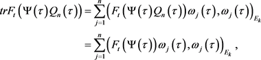
where $\Lambda$ is the cross product, $tr$ represents the trace of the operator, $Q_n\left(\tau \right)$ represents the orthogonal projection from to.

For a given time, we set. is the standard orthogonal basis of the space .

Define the scalar product in as follows

From the above, we have

where

where.

There exists a positive constant r, such that

Due to is the standard orthogonal basis of the space.

Almost to all t, we arrive at

where and, is the eigenvalue of and.

So,

Setting

Therefore,

Thus, the Lyapunov exponent of is uniformly bounded.

From what has been discussed above, we get

Thus,

n

4. Conclusion

In this paper, a class of high order Kirchhoff type equation has been investigated. In recent years, much work concerning the low order Kirchhoff type equation has been published. However, to the best of my knowledge, there were few long-time behaviors for the high order Kirchhoff type equation with strong damping. We have proved the existence and uniqueness of the global solution of the problem by using prior estimates and the Galerkin’s method under proper assumptions for the rigid term. Furthermore, we have been obtained the Hausdorff dimension and Fractal dimension of the family of global attractors.

Acknowledgements

The authors express their sincere thanks to the aonymous reviewer for his/her careful reading of the paper, giving valuable comments and suggestions. These contributions greatly improved the paper.

Authors’ Contributions

The work was realized by the author. The author read and approved the final manuscript.

Conflicts of Interest

The authors declare no conflicts of interest.

References

[1]	Ladyzhenskaya, O.A. and Seregin, G.A. (1999) On Partial Regularity of Suitable Weak Solutions to the Three-Dimensional Navier—Stokes Equations. Journal of Mathematical Fluid Mechanics, 1, 356-387. https://doi.org/10.1007/s000210050015
[2]	Ladyzhenskaya, O.A. (1988) Attractors of Nonlinear Evolution Problems with Dissipation. Journal of Soviet Mathematics, 40, 632-640. https://doi.org/10.1007/BF01094189
[3]	Ladyzhenskaya, O.A. (1985) Finite-Dimensionality of Bounded Invariant Sets for Navier-Stokes Systems and Other Dissipative Systems. Journal of Soviet Mathematics, 28, 714-726. https://doi.org/10.1007/BF02112336
[4]	Temam, R. (1990) Inertial Manifolds. The Mathematical Intelligencer, 12, 68-74. https://doi.org/10.1007/BF03024036
[5]	Foias, C., Sell, G.R. and Temam, R. (1988) Inertial Manifolds for Nonlinear Evolutionary Equations. Journal of Differential Equations, 73, 309-353. https://doi.org/10.1016/0022-0396(88)90110-6
[6]	Sell, G.R. and You, Y.C. (1992) Inertial Manifolds: The Non-Self-Adjoint Case. Journal of Differential Equations, 96, 203-255. https://doi.org/10.1016/0022-0396(92)90152-D
[7]	Guo, B.L. (2000) The Infinite Dimension System. National Defense Industry Press, Beijing.
[8]	Chueshov, I., Lasiecka, I. and Toundykov, D. (2009) Global Attractor for a Wave Equation with Nonlinear Localized Boundary Damping and a Source Term of Critical Exponent. Journal of Dynamics and Differential Equations, 21, Article No. 269. https://doi.org/10.1007/s10884-009-9132-y
[9]	Yang, Z.J. and Wang, Y.Q. (2010) Global Attractor for the Kirchhoff Type Equation with a Strong Dissipation. Journal of Differential Equations, 249, 3258-3278. https://doi.org/10.1016/j.jde.2010.09.024
[10]	Gao, Y.L., Sun, Y.T. and Lin, G.G. (2016) The Global Attractors and Their Hausdorff and Fractal Dimensions Estimation for the Higher-Order Nonlinear Kirchhoff-Type Equation with Strong Linear Damping. International Journal of Modern Nonlinear Theory and Application, 5, 185-202. https://doi.org/10.4236/ijmnta.2016.54018
[11]	Lin, G.G. (2011) Nonlinear Evolution Equations. Yunnan University Press, Kunming.
[12]	Kirchhoff, G. (1883) Vorlesungen Uber Mechamic. Tauber, Leipzig.
[13]	Yang, Z.J. and Da, F. (2018) Stability of Attractors for the Kirchhoff Wave Equation with Strong Damping and Critical Nonlinearities. Journal of Mathematical Analysis and Applications, 469, 298-320. https://doi.org/10.1016/j.jmaa.2018.09.012
[14]	De Brito, E.H. (1987) Nonlinear Initial Boundary Value Problems. Nonlinear Analysis: Theory, Methods & Applications, 11, 125-137. https://doi.org/10.1016/0362-546X(87)90031-9
[15]	Matsuyama, T. and Ikerata, R. (1996) On Global Solutions and Energy Decay for the Wave Equations of Kirchhoff Type with Nonlinear Damping Terms. Journal of Mathematical Analysis and Applications, 204, 729-753. https://doi.org/10.1006/jmaa.1996.0464
[16]	Ono, K. (1997) On Global Solutions and Blow-Up Solutions of Nonlinear Kirchhoff Strings with Nonlinear Dissipation. Journal of Mathematical Analysis and Applications 216, 321-342. https://doi.org/10.1006/jmaa.1997.5697
[17]	Yamada, Y. (1982) On Some Quasilinear Wave Equations with Dissipative Terms. Nagoya Mathematical Journal, 87, 17-39. https://doi.org/10.1017/S0027763000019929
[18]	Bozhkov, Y. and Dimas, S. (2013) Group Classification and Conservation Laws for a Two-Dimensional Generalized Kuramot—Sivashinsky Equation. Journal of Nonlinear Analysis, 84, 117-135. https://doi.org/10.1016/j.na.2013.02.010
[19]	Autuori, G., Pucci, P. and Salvatori, M.C. (2009) Asymptotic Stability for Nonlinear Kirchhoff Systems. Nonlinear Analysis: Real World Applications, 10, 889-909. https://doi.org/10.1016/j.nonrwa.2007.11.011
[20]	Yang, Z.J. (2007) Longtime Behavior of the Kirchhoff Type Equation with Strong Damping on RN. Journal of Differential Equations, 242, 269-286.
[21]	Wu, S.T. and Tsai, L.Y. (2006) Blow-Up of Solutions for Some Nonlinear Wave Equations of Kirchhoff Type with Some Dissipation. Nonlinear Analysis: Theory, Methods & Applications, 65, 243-264. https://doi.org/10.1016/j.na.2004.11.023
[22]	Chueshov, I. (2011) Long-Time Dynamics of Kirchhoff Wave Models with Strong Nonlinear Damping. Journal of Differential Equations, 252, 1229-1262. https://doi.org/10.1016/j.jde.2011.08.022
[23]	Lin, G.G. and Li, Z.X. (2019) A Class of Higher Order Nonlinear Kirchhoff Equation Attractor Family and Its Dimension. Journal of Shandong University (Science Edition), 54, 1-11.