Practical Meta-Reinforcement Learning of Evolutionary Strategy with Quantum Neural Networks for Stock Trading

Erik Sorensen, Wei Hu

Department of Computer Science, Houghton College, Houghton, NY, USA.

DOI: 10.4236/jqis.2020.103005                

Abstract

We show the practicality of two existing meta-learning algorithms Model- Agnostic Meta-Learning and Fast Context Adaptation Via Meta-learning using an evolutionary strategy for parameter optimization, as well as propose two novel quantum adaptations of those algorithms using continuous quantum neural networks, for learning to trade portfolios of stocks on the stock market. The goal of meta-learning is to train a model on a variety of tasks, such that it can solve new learning tasks using only a small number of training samples. In our classical approach, we trained our meta-learning models on a variety of portfolios that contained 5 randomly sampled Consumer Cyclical stocks from a pool of 60. In our quantum approach, we trained our quantum meta-learning models on a simulated quantum computer with portfolios containing 2 randomly sampled Consumer Cyclical stocks. Our findings suggest that both classical models could learn a new portfolio with 0.01% of the number of training samples to learn the original portfolios and can achieve a comparable performance within 0.1% Return on Investment of the Buy and Hold strategy. We also show that our much smaller quantum meta-learned models with only 60 model parameters and 25 training epochs have a similar learning pattern to our much larger classical meta-learned models that have over 250,000 model parameters and 2500 training epochs. Given these findings, we also discuss the benefits of scaling up our experiments from a simulated quantum computer to a real quantum computer. To the best of our knowledge, we are the first to apply the ideas of both classical meta-learning as well as quantum meta-learning to enhance stock trading.

Keywords

Reinforcement Learning, Deep Learning, Meta-Learning, Evolutionary Strategy, Quantum Computing, Quantum Machine Learning, Stock Market, Algorithmic Trading

1. Introduction

Profitable stock trading is vital to investment companies. In order for stock trading to be profitable, an investment strategy must be in place to maximize performance, which can be measured in expected return. However, many different factors must be considered to measure expected return, such as future estimated value or risk of loss, which makes it difficult for market analysts to make quick decisions about how to trade their many stocks profitably in their portfolios.

The problem of trading profitably on the stock market has been solved with some success with the recent developments of Deep Reinforcement Learning (DRL) [1]. This method treats the stock market as a Markov Decision Process (MDP) where the algorithm sees only the data currently available to it and makes a decision based strictly on that data [2]. Similar algorithms have been created that not only use stock market data but other data as well, such as sentiment data from Twitter [3].

One of the largest issues with training deep learning algorithms to trade on the stock market is that once they have successfully learned to trade a certain set of stocks, that learning does not translate to other stocks, even if those stocks are very similar to the ones it has previously learned. This problem is called overfitting, and is one of the biggest hurdles in training DRL models [4]. Because of overfitting, in order for a DRL algorithm to learn to trade a new set of stocks, it has to completely forget what it has learned before and spend extra time training on this new set of stocks. This can cause problems if a trading firm wants to update a portfolio it has with new stocks in a short amount of time. The time the algorithm spent training on the old portfolio is now completely wasted, which could be time the algorithm is maximizing returns and making profits on the stock market.

In order to solve this problem, we propose a novel meta-learning approach to trading on the stock market. Meta-learning is a field of reinforcement learning that enables the learning agent to generalize previous knowledge to similar areas it has learned before which enables it to learn new environments with very little training time. We propose to use the meta-learning algorithms Mo- del-Agnostic Meta-Learning (MAML) [5] and Fast Context Adaption Via Meta- learning (CAVIA) [6] to learn how to trade on new but similar portfolios with much less training. To the best of our knowledge, we are the first to apply meta-learning techniques to enhance stock trading.

Furthermore, the stock market is a very complex environment with many variables at play and classical computers can struggle to learn effectively with this much data. The recent developments of Quantum Computing is a promising solution to train an algorithm quickly on the large amounts of data the stock market provides, which has the potential to increase our performance when trading. With these exciting developments in mind, we also explore quantum implementations of the meta-learning algorithms MAML and CAVIA on a simulated quantum machine using our novel quantum algorithms Q-MAML and Q-CAVIA. To the best of our knowledge we are also the first to create quantum meta-learning algorithms. In summary our main contributions of this paper are as follows:

· We provide a new way to increase training performance when learning new stock portfolios via meta-learning.

· We create new quantum implementations of these meta-learning algorithms used to enhance stock trading.

· As far as we know, we are the first to explore both meta-learning to enhance stock trading and the first to create a quantum implementation of the meta-learning algorithms MAML and CAVIA.

2. Background

In this section we give a brief background in the fields of reinforcement learning, evolutionary strategies, meta-learning, and continuous variable quantum computing.

2.1. Reinforcement Learning

Reinforcement learning (RL) is one area of machine learning in which an agent interacts with an environment to learn how to maximize rewards by taking certain actions within that environment [7]. The goal of RL is to find a policy, which describes which actions to take in certain states, that maximizes the reward. More concretely, a policy ( $\pi$ ) is a probability distribution that maps states $s\in \mathcal{S}$ to actions $a\in \mathcal{A}$, or stated differently $\pi \mathrm{<mo>\; :\; </mo>}\mathcal{A}\times \mathcal{S}\to \left[\mathrm{0,1}\right]$. Each task in RL is a MDP which contains a tuple ${\mathcal{T}}_i=\left(\mathcal{S}\mathrm{,}\mathcal{A}\mathrm{,}r\mathrm{,}q\mathrm{,}{q}_0\right)$, where $\mathcal{S}$ is a set of states, $\mathcal{A}$ is a set of actions, $r\left(s_t\mathrm{,}{a}_t\mathrm{,}{s}_{t+1}\right)$ is a reward function, $q\left(s_{t+1}\mathrm{<mo>\; |\; </mo>}{s}_t\mathrm{,}{a}_t\right)$ is a transition function which gives the probability of moving from $s_t$ to $s_{t_1}$ by doing action $a_t$ at time t, and $q_0\left(s_0\right)$ is an initial state distribution. The optimal policy is a policy that receives the greatest cumulative reward $\mathcal{J}$ under $\pi$,

$\mathcal{J}\left(\pi \right)={\mathbb{E}}_{q_0\mathrm{,}q\mathrm{,}\pi }\left[{\displaystyle \underset{t=0}{\overset{H-1}{\sum }}}{\gamma }^{t}r\left(s_t,a_t,s_{t+1}\right)\right]$ (1)

where $H\in \mathbb{N}$ is the horizon and $\gamma \in \left[\mathrm{0,1}\right]$ is the discount factor which determines how much the agent cares about rewards in the distant future relative to those in the immediate future.

RL is very useful, especially when we are trying to learn complicated environments that would be too difficult to write instructions for by hand. By only defining the rewards the agent will seek, it will teach itself how to best navigate the environment and maximize its reward. All methods of RL have this same goal, which is to find the optimal policy to maximize reward.

RL algorithms that use neural networks are defined as Deep Reinforcement Learning algorithms. Neural networks are a technique of function approximation that can learn continuously complex environments faster and more effectively. Neural Networks are able to do this via activation functions which enables them to learn on these more complex environments [8].

2.2. Evolution Strategies

Evolutionary Strategies (ES) are an alternative to Stochastic Gradient Descent to optimize deep learning models. These strategies were created from the family of Evolutionary Algorithms (EA). The idea behind these algorithms is to mimic what natural selection does to species in biology. Over time, natural selection works by naturally propagating “good” genes. Organisms that have these “good” genes are more likely to survive from predators and perpetually pass these genes to their offspring. This cycle continues until all the organisms of the species have these “good” genes.

We can apply this same idea of natural selection to optimize a deep learning model. Recall that in deep learning, the goal is to reach the optimal policy that receives the greatest cumulative reward by updating the parameters of the neural network. In other words, we can find the optimal configuration of parameters $\theta$ to find the optimal policy $\pi$ for any state x, which is described as $\pi \left(x\right)$. 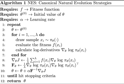This alternative way for optimizing parameters is shown in Algorithm 1 [9].

There are a few important lines to note in Algorithm 1. First, we apply a “jitter” to each of the samples from step 4. The “jitter” is created through random variance based on a hyper parameter, $\sigma$, which controls how much random variance we have in “jittering”. Then, based on the samples chosen with this random variation we can evaluate the fitness of them in line 5 in accordance with our fitness function f at state $x_i$, and then perform our update to our parameters $\theta$ toward the optimal policy $\pi$ via the computed log-derivatives shown in step 9.

Furthermore, ES is effective for deep reinforcement learning. It has been

shown that ES scales very well with multiple CPUs for parallelization, even with up to 1000 CPUs [10]. This allows us to train deep networks to solve complicated environments in a short amount of time. ES has also been found to be a great black box optimization technique because it is not impacted by delayed rewards, does not require value function approximation, and does not need temporal discounting, which all cause problems to train an agent on a complex environment. These factors make ES effective for deep reinforcement learning.

2.3. Meta-Reinforcement Learning

Reinforcement Learning struggles with the problem of overfitting, or learning one task very well while failing to generalize what it has learned to other tasks, even ones that are very similar. One of the things that humans can do very well is generalize things that they have learned previously to new tasks. One such example is that once a human learns to ride a bicycle, it takes little or no instructions to figure out how to ride a motorcycle. These two tasks are very similar in practice, and our human minds can automatically detect the similarities between these two tasks and transfer our previous knowledge to learn the new task quickly. This is impossible to do for traditional RL algorithms, which require completely different training sessions for each individual task, even if the two tasks are very similar.

The field of meta-reinforcement learning hopes to solve this problem. The goal of meta-reinforcement learning is to create good models that are capable of adapting or generalizing to new tasks and environments that it never encountered during training time. In order to adapt to these new tasks, the meta-rein- forcement learning algorithm is shown small batches of this new task with limited exposure. Eventually, the algorithm will be able to perform well on this new task with much less training. The research field of meta-learning is very broad whose goal is to learn how to learn, but for the purposes of our paper, whenever we say meta-learning we mean meta-reinforcement learning, which applies meta-learning ideas to reinforcement learning algorithms.

Some examples of how meta-learning could be used in the real world are:

· A image classifier trained to detect cat images can learn to detect non-cat images quickly with only a few images [11].

· A game bot learning to play checkers after it has already learned chess.

· A meta learned regression algorithm can learn shapes of new sine curves with only seeing a few of them [5].

The goal of few-shot meta-learning, or learning with very few training steps, is to enable the agent to quickly discover the optimal policy for a new task using only a small amount of experience from the new test setting. However, gradient-based optimization is designed to work with large sample sizes, not the small amount of training required for meta-learning to take place. MAML and CAVIA are two algorithms that look to solve this problem using the optimization approach for meta-learning.

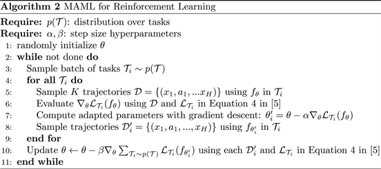
2.3.1. MAML

MAML stands for Model-Agnostic Meta-Learning and its purpose is to be a general meta-learning algorithm that is compatible with all models that use some form of gradient descent to update learning parameters [5]. It is used in reinforcement learning to accelerate the learning for neural network policies when the agent only has a little bit of exposure to the new environment. The idea behind MAML is to use two separate training loops, an inner loop (lines 4 - 9 in Algorithm 2) that learns task specific knowledge updating a set of parameters ${\theta }^{\prime }$, and an outer loop (lines 2 - 11 in Algorithm 2) that learns global knowledge across tasks updating another set of parameters $\theta$ based on the task specific parameters ${\theta }^{\prime }$ for each training batch of tasks. Therefore, we can use the $\theta$ to quickly learn new tasks that are similar to the tasks ${\theta }^{\prime }$ were trained on. The complete algorithm for MAML for reinforcement learning is shown in Algorithm 2.

MAML has been shown to be a successful way to quickly train a model on a variety of popular reinforcement learning environments such as the 2D Navigation environment and the complex MuJoCO 3D quadruped environment. In both cases, MAML achieved the desired goal for both environments with only a few training iterations [5].

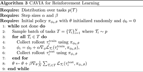
2.3.2. CAVIA

Fast context adaptation via meta-learning, or CAVIA, is an extension of MAML which claims to be less prone to meta-overfitting, which has been shown to be a problem for MAML [12], is easier to parallelise, and is more interpretable. This is done by splitting the model parameters into two parts: the context parameters which are used as an additional input to the model and are adapted to individual tasks, and shared parameters that are meta-trained and shared across all tasks. The context parameters are also only updated during test time which leads to a low-dimensional task representation which boosts performance during training.

In MAML, the gradients of the model parameters $\theta$ are calculated before the inner-loop update, which means that the outer-loop update involves a higher order derivative of $\theta$. This increases complexity of the algorithm and decreases performance while training. CAVIA removes the higher order derivative calculation

by adding the context parameters $\varphi$ which are calculated within the inner loop for each task, and is separate from the model parameters $\theta$ which are meta-leaned and calculated in the outer loop and shared across tasks. This is done by updating the model parameters $\theta$ with the average of the context parameters $\varphi$, which means that the higher order gradients are already included in $\theta$ due to its dependence on $\varphi$. The full algorithm can be found in more detail in Algorithm 3 [6].

2.4. Continuous Variable Quantum Computing

A recently popular model of quantum computing is continuous variable (CV) quantum computing which serves as a continuous method of computation and leverages wavelike properties found in nature where quantum information is not encoded in bits but in the quantum states of fields, such as the electromagnetic field. The particles that encode this information are called qumodes, which carry more information than bits and are more powerful due to their quantum properties. For example, qumodes can be in a quantum superposition of multiple states at the same time. The state of the qumodes are manipulated using quantum gates and multiple gates applied successively to qumodes make up a quantum algorithm.

Qumodes can be represented by the wavefunction representation, where we specify a single continuous variable, say x, and represent the state of the qumode through a complex-valued function of this variable called the wavefunction $\psi \left(x\right)$. The single continuous variable x can also be interpreted as a position coordinate, and ${\left|\psi \left(x\right)\right|}^2$ as the probability density of a particle (photon) being located at x. Based on elementary quantum theory, we can use a wavefunction based on a conjugate momentum variable, $\varphi \left(p\right)$. The position x and the momentum p can also be pictured as the real and imaginary parts of a quantum field, such as light [13]. A physical model of one of these computers consists using optical systems [14] in the microwave regime [15] and using ion traps [16].

The CV model is largely unexplored when it comes to machine learning, but there have been some recent research that have shown the usefulness of the continuous nature of a CV quantum circuit being used as a kernel-based classifier [17]. Even more promising is the use of CV quantum circuits to create neural

networks [13]. The CV model is a good fit to create neural networks due to them being continuous in nature. Neural networks are the most expensive part computationally of RL algorithms and Quantum neural networks aim to speed up computation time exponentially when run on a quantum computer.

A quantum neural network is made with a specific set of quantum gates that manipulate qumodes as they pass through them. Gates can either be Gaussian or not. Gaussian gates are the “easy” operations for a CV quantum computer. The rotation $R\left(\varphi \right)$, displacement $D\left(\alpha \right)$, and squeezing $S\left(r\right)$ gates are Gaussian operations and are applied to one qumode. Another Gaussian gate, called beam- splitter $BS\left(\theta \right)$, can be understood as a rotation between two qumodes. These gates can be represented as matrix transformations on phase space and are as follows,

$R\left(\varphi \right)\mathrm{<mo>\; :\; </mo>}\left[\begin{array}{c}x\\ p\end{array}\right]\mapsto \left[\begin{array}{cc}cos\left(\varphi \right)& sin\left(\varphi \right)\\ -sin\left(\varphi \right)& cos\left(\varphi \right)\end{array}\right]\left[\begin{array}{c}x\\ p\end{array}\right]\mathrm{,}$

$D\left(\alpha \right)\mathrm{<mo>\; :\; </mo>}\left[\begin{array}{c}x\\ p\end{array}\right]\mapsto \left[\begin{array}{c}x+Re\left(\alpha \right)\\ p+Im\left(\alpha \right)\end{array}\right]\mathrm{,}$

$S\left(r\right)\mathrm{<mo>\; :\; </mo>}\left[\begin{array}{c}x\\ p\end{array}\right]\mapsto \left[\begin{array}{cc}{\text{e}}^{-r}& 0\\ 0& {\text{e}}^r\end{array}\right]\left[\begin{array}{c}x\\ p\end{array}\right]\mathrm{,}$

$BS\left(\theta \right)\mathrm{<mo>\; :\; </mo>}\left[\begin{array}{c}{x}_1\\ x_2\\ p_1\\ p_2\end{array}\right]\mapsto \left[\begin{array}{cccc}cos\left(\theta \right)& -sin\left(\theta \right)& 0& 0\\ sin\left(\theta \right)& cos\left(\theta \right)& 0& 0\\ 0& 0& cos\left(\theta \right)& -sin\left(\theta \right)\\ 0& 0& sin\left(\theta \right)& cos\left(\theta \right)\end{array}\right]\left[\begin{array}{c}{x}_1\\ x_2\\ p_1\\ p_2\end{array}\right]\mathrm{.}$

The ranges for the parameter values are $\varphi \mathrm{,}\theta \in \left[\mathrm{0,2}\pi \right]$, $\alpha \in ℂ\cong {ℝ}^2$ and $r\in ℝ$. To help visualize what these Gaussian transformations do, we can map the phase space as a quasi probability density, therefore simulating what each of the gates look like when they are applied to a qumode.

One more non-Gaussian gate is used to build quantum neural networks, the Kerr gate which is represented by the function $K\left(\kappa \right)=\text{exp}\left(i\kappa {\hat{n}}^2\right)$. A universal gate set for CV quantum computing consists of all of the Gaussian transformations shown above, and one non-Gaussian gate such as the Kerr gate. With a universal gate set, we can approximate any function with CV quantum computing. This universal gate set is visualized in Figure 1. Parallels can be drawn to classical neural networks, where the Gaussian gates are the same as linear transformations in classical neural networks and the non-Gaussian gates are non-linear transformations.

These gates can then make up a neural network algorithm that is similar to how classical neural networks operate. We can use these quantum neural networks in place of the classical neural networks to speed up computation time on a quantum computer. In the future, we could use a classical computer to run the RL algorithms together with a quantum chip that runs quantum gate operations to compute the neural networks very quickly [18].

Figure 1. These images, in order, are the vacuum state, which is the initial state of the qumodes with no gate applied, the rotation gate, the displacement gate, the squeezing gate, and the Kerr Gate. These visualizations show the probability of photons location and momentum in phase space. Location and momentum make up each axis while the peaks of green show high probabilities of photons being at that location and momentum, and red shows low probabilities. The quantum gates manipulate this probability distribution of the photons in phase space. Note how the Kerr gate can achieve negative probabilities [13].

3. Problem Statement

Instead of trying to teach a reinforcement learning agent to master a game on the Atari, which is a very popular and standard way to benchmark RL performance, we are going to train a RL agent to trade on the stock market. The stock market is an attractive alternative environment for testing RL performance because it offers a more practical application for learning than playing a video game. Also, all of the data on the stock market is publicly available and easily accessible. The goal of this paper is to not create an algorithm to make a lot of money on the stock market but to show how a combination of reinforcement learning, meta learning, and quantum computing can effectively learn to trade on a practical environment like the stock market.

In our paper, we will train an agent to manage m multiple portfolios at the same time, each with n number of stocks. Then, using meta reinforcement learning our agent will learn to trade a single portfolio that contains completely different stocks than what it has learned to trade with before with much less training required.

In order to train the RL agent we must model the stock trading process as a MDP which is the baseline assumption required for all of the RL methods described above. This frames the problem as a maximization problem, where the goal of the RL agent is to maximize the amount of trading profits it will receive when trading on the stock market. Figure 2 shows what this MDP looks like. This MDP includes:

· State $s=m_t$ : which includes a vector of size $n+1$, where n is the number of stocks in the portfolio plus 1 for the amount of total cash we hold. The closing prices $p\in ℝ$ for all of the stocks in each portfolio m have time-step measure t, where t denotes the day we are trading.

· Action a: which is the action the agent can perform on each portfolio m. The actions are encoded by the portfolio weights $w_t\in \left[\mathrm{0,1}\right]$ which describe the percentage amount each stock makes up the portfolio at each timestep t where the sum of all $w_t$ in the portfolio m is 1.

· Reward $r\left(s\mathrm{,}a\mathrm{,}{s}^{\prime }\right)$ : which is the change of the portfolio value when action a

Figure 2. As the stock price changes from s to $s^{\prime }$, action a is taken which is encoded as portfolio weights $\left(w_0\mathrm{,}{w}_1\mathrm{,}{w}_2\mathrm{,}\cdots \right)$ chosen by the agent, leading to the next portfolio value. All of the portfolio weights sum up to one.

is taken at state s and arrives at the new state $s^{\prime }$. The total portfolio value is the sum of the closing prices in all held stocks in the portfolio plus the total remaining cash we are holding that is not put in stocks. The goal of the agent is to maximize r for a given time frame.

· Policy $\pi \left(s\right)$ : which denotes the trading strategy of stocks at state s, which is the probability distribution of a at state s.

· Action-value function $Q_{\pi }\left(s\mathrm{,}a\right)$ : which is the expected reward achieved by action a at state s following policy $\pi$.

Each portfolio is composed of a vector of weights $w_t\in \left[\mathrm{0,1}\right]$, which describes how much percentage the portfolio is composed of each asset at timestep t. These weights are then the output of our agent, and how it decides how much of each asset in the portfolio to hold, which always sum up to one by definition, ${\displaystyle {\sum }_i}{w}_t,i=1$. The first weight is special as it describes how much cash is being held. At timestep 0, the cash weight is always 1 because no trading has occurred yet so all of our assets are in cash. The rate of return at timestep t is then:

$p_t:=y_t\cdot w_{t-1}-1$ (2)

where at time t, $p_t$ is the rate of return of the portfolio, $y_t$ is the vector of closing prices of each stock in the portfolio, and $w_t$ is the assigned vector of weights by the agent. The corresponding logarithmic rate of return is

$r_t:=\ln y_t\cdot w_{t-1}.$ (3)

The logarithmic rate of return is used to normalize the reward function so that it is easier for the agent to learn. This ensures that when the model goes to update its gradients, that the gradients all get updated on the same scale. This makes training more stable which should also increase performance of our model.

If there is no transaction cost, the final portfolio value will be

$p_f=p_0\exp \left({\displaystyle \underset{t=1}{\overset{t_f+1}{\sum }}}{r}_t\right)=p_0{\displaystyle \underset{t=1}{\overset{t_f+1}{\prod }}}{y}_t\cdot w_{t-1},$ (4)

where $p_0$ is the initial investment amount. The goal of the reinforcement learning agent is to maximize the portfolio value $p_f$ for a given time frame.

Assumptions

In this work, only back-test tradings are considered. This means that our model pretends to be “back in time” at a point in market history and then trades on unknown “future” market data. In order to perform backtesting we must make a couple of assumptions:

1) Zero slippage: The liquidity of all market assets is high enough that each trade can be carried out immediately at the last price when an order is placed. This also includes the ability to always place orders immediately at the end of the day.

2) Zero market impact: The capital invested by the agent is insignificant enough to not influence the market.

In a real-world trading environment, if the volume in the market is high enough, then these two assumptions are near to reality. The Consumer Cyclical stocks that we will be trading are all high volume stocks so our assumptions are justified. Furthermore, we assume that there are no transaction costs to trading. In the modern world of stock trading there are many online brokerages that offer no cost trading, several of which are Robinhood, Fidelity, and E-Trade. Since we will only trade stocks once per day we can assume no transaction costs will be charged if one of these online brokerages are used.

4. Related Works

Algorithmic trading on the stock market is a very active research domain. Here we will focus on those algorithms which use different deep reinforcement learning techniques.

One deep reinforcement learning strategy used a Portfolio-Vector Memory (PVT) technique to form the problem as optimizing a portfolio of assets, where each asset in the portfolio has an assigned weight given to it by the learning agent [19]. The learning agent was then constructed using a Convolutional Neural Network (CNN), a basic Recurrent Neural Network (RNN) and Long Short-Term Memory (LSTM). Our research used a similar method to form the trading problem using the portfolio of asset weights, but differed in how the learning agent was constructed. Their method also learned to trade a portfolio of Cryptocurrencies, while we focus on stocks in the New York Stock Exchange (NYSE).

Utilizing quantum computing for algorithmic trading is a new field of research but is increasing in activity. One method explores using a Quantum-ins- pired tabu search to find trading rules that will optimize profits when trading on the stock market [20]. This research uses quantum states to intensify the search for these optimal trading rules, which allows it to more effectively explore the stocks in the market, avoiding negative results. This research is one of the few that explores using quantum states to find optimal trading strategies, but differs from our research as it does not explore using quantum neural networks and a reinforcement learning technique to find an optimal trading strategy.

Another branch of algorithmic trading with quantum computers explores using quantum artificial neural networks (QuANNs) as a way to build and simulate financial market models with adaptive selection of trading rules [21]. The idea is that QaANNs can build a model of financial market dynamics that incorporates quantum interference and quantum adaptive computation in the probabilistic description of financial returns. While this field of research is still in its early stages, this research shows that QuANNs are able to successfully model financial markets and bridge the fields of financial dynamics and risk modeling. In our research, we also use a form of quantum neural networks, but ours is modeled after the continuous form of quantum computing, while this research uses discrete quantum computing.

At the time of writing, there is no current research that uses continuous quantum neural networks to learn to trade on financial markets. Furthermore, there is also no research that looks into applying the field of meta-learning algorithms to better improve the agent’s learning of financial markets. Our research is the first to combine both the fields of meta-learning and continuous quantum neural networks to teach an agent to trade on financial markets.

5. Methods

5.1. Data Treatments

Our trading experiments were done on stocks that are classified as Consumer Cyclical (CC) stocks. Consumer Cyclical is a category of stocks that rely heavily on the business cycle and economic conditions. It includes industries such as automotive, housing, entertainment, and retail.

We extracted a total of 60 different CC stocks from finance.yahoo.com. In our experiments, our agents trained on m multiple portfolios, each having a vector of size n + 1, where n is the number of stocks inside the portfolios and where n + 1 includes the amount of cash the agent has available to purchase stocks with. To fill the portfolios during training time, we randomly sample n stocks from 55 of the 60 stocks available. The random sampling is done so that the meta-lear- ning algorithm learns how to trade CC stocks as a whole and not just individual stocks. For our classical experiments m and n were set to 5. This means that our agent trained on 5 different portfolios, each containing 5 randomly chosen CC stocks.

We then split this data into a training set that contains the first 70% of the data and a testing set that contains the last 30% of the data. Then, to test our agents performance, we train the agent with only a few training iterations on 1 portfolio that contains the last 5 of the stocks that were not included in the random sampling during training. This test portfolio contained the same set of CC stocks across all tests. These stocks were ABC, AKAM, APD, AVP, and BAC. The test portfolio data is also split with the same 70/30 train/test split like the training set. We then meta-train the agent with only a few training iterations on the 70% test set, and then run a back test on the last 30% of the test portfolio to validate the performance of the agent on data it has not seen before. Back testing is a standard way to measure how well a strategy or model would have done at some time period in the past. In our case, our period of back testing is our 30% split of our testing dataset. The stock data we used were from the dates 1/2/2001 to 6/12/2002. Therefore, with the 70/30 train/test spit described above, the agent trained on stock data from 1/2/2001 to 1/4/2002 and was back-tested on stock data from 1/7/2002 to 6/12/2002. This is shown in Figure 3. It is important to note that the data we have contains only days the stock market is open, which is most week days (Monday through Friday) excluding any major holidays.

Like mentioned before, each portfolio is a vector of size n + 1 where n is the number of stocks in the portfolio plus one for the amount of cash the agent currently has to trade with. The data available to us for each day includes the opening price, the highest price in the day, the lowest price in the day, the closing price of the day, and the volume or the amount of stock traded in the day. In order to make the problem simpler and to reduce the total amount of data the agent needs to process to make training time quicker, we only use the closing price of the day. While giving the agent more data to train on has the potential to increase its trading performance, for the purposes of this paper, we think that the closing price offers enough information to show the potential of meta-learning on trading on the stock market. Future work could include using more data to further boost performance.

In order for the agent to more effectively learn from the data, we group multiple days together as one input into the model. We do this because it would be near impossible for the model to make a decision from just one days closing price. With only one days worth of information, the model doesn’t know if the stock price is going up or down and therefore cannot make a judgement on if its a good time to purchase the stock in order to make a profit. To solve this, we input ws stocks at a time, where ws is called the window size. In our experiments, the window size is 10. This means that at every timestep t, the agent is given the data from the past 10 days from t, or t − 9, for each of the stocks in the portfolio, which can be seen in Figure 4. This makes the size of the input data

Figure 3. Data Splitting.

Figure 4. For each training iteration, the input data shifts to include the last 10 days of data from the current timestep t.

for each day of training m × n × ws.

Another very common strategy to improve the stability of learning is to normalize the data that it receives so that variation between the data is reduced. In order to do this, we apply two strategies. First, we have selected to train and test only on stocks that have a price between $0 and $50. This way, there are no very large stocks that could cause a high variance in training our model. Second, we also normalize our data by using the logarithmic rate of return shown in Equation (3).

5.2. Two Classical Models for Meta Stock Trading

In this section, we will discuss how our models were created and how learning takes place. We have a total of 4 algorithms being tested: MAML, CAVIA, and our quantum implementations of these algorithms Quantum MAML (Q-MAML) and Quantum CAVIA (Q-CAVIA). All of these algorithms use the NES model for updating the gradients. Normally, MAML and CAVIA use gradient descent to update the gradients, but they are both general purpose meaning that any method to update the gradients of our model parameters will work. We chose to use the NES algorithm to replace the derivative calculations in MAML and CAVIA because it is has been shown to avoid overfitting and scales well with parallel computing [10]. We will then compare our model’s performances in the next section and discuss the benefits for using these models.

In our implementation of MAML and CAVIA using NES, we have a neural network with 2 hidden layers of size 50 × 100 and 500 × 500, and an input layer of size 1 × 50 and an output layer of size 500 × 5 + 1 (see Figure 5). The outputs are encoded with a softmax so that our final outputs are a vector of portfolio weights where each weights value is between 0 and 1 and the sum of all of the portfolio weights equals 1. Each of these numbers describes how much cash and how much of each stock we should hold as a percentage of our portfolio for that day of trading. Each of the parameters in the hidden layers of our neural network then act like a voting system, where each of them contribute weight for each item in the portfolio weight vector.

Figure 5. NES neural network implementation for stock trading: This is a realization of how the inputs for one portfolio are mapped to outputs in our model. The inputs include the closing prices of all n stocks where ws is our window size which we have set to 10. Then the inputs are applied to the weights of our neural network with a linear activation function (matrix multiplication). The last step we add a cash bias and apply the softmax function which maps the neural network weights to a portfolio vector of size m + 1. This means that each item in the vector is the agents decision of the percentage of each asset to hold at the current timestep.

The NES algorithm updates each of these weights following Algorithm 1, where our fitness function f is the reward function, or the expected portfolio value, our learning rate is set to 0.03, our $\sigma$ which applies the “jitter” is set to 0.1, and our population size is set to 15.

Our goal in meta-learning is not to learn to trade one portfolio, but to learn how to trade CC stocks as a whole. Because of this, our training loop trains on 5 separate portfolios, each containing 5 CC stocks. In order to do this, we loop through each portfolio, updating our agents parameters on each portfolio one at a time. This means we have one set of parameters for all of our portfolios. Training in this way makes the training essentially maximize the reward over all of the stocks, or in other words, it learns the average best policy for all of the portfolios that contain CC stocks. We do this for 2500 epochs, meaning that we train the algorithm over each portfolio 2500 times. We chose 2500 epochs because training progress slowed down significantly around this point.

Then, we train the meta-algorithm on 1 previously unseen portfolio with only 20 epochs, which is significantly less epochs required than during training time. How the meta-algorithm is trained is different for each MAML and CAVIA algorithms.

5.2.1. Training MAML for Stock Trading

The MAML algorithm requires a separate set of model parameters ${\theta }^{\prime }$ to be trained separately along with the main parameters $\theta$. In our implementation ${\theta }^{\prime }$ is initialized with the same structure as the normal parameters and they are also updated via the NES algorithm. The difference between these parameters is when they are updated. After each $\theta$ parameter is updated for each of the portfolios, we save the gradients from each of these updates. We then use each of these gradients from $\theta$ to update our meta-gradients which are then used to update our meta-parameters ${\theta }^{\prime }$. These parameters are then used to speed up our training on our new unseen test portfolio, which only requires around 20 epochs to learn.

In summary, MAML requires two different gradients to be computed which increases computational complexity due to having to compute 2^nd order gradients. This is done to train the ${\theta }^{\prime }$ parameters which are essentially an average of the normal $\theta$ parameters and are used to dramatically increase training speed on an environment that is similar to what the $\theta$ parameters were trained on.

5.2.2. Training CAVIA for Stock Trading

CAVIA aims to increase the performance of MAML by taking away the 2nd order gradients and replacing it with context parameters $\varphi$. The context parameters are initialized with a vector of size 5, which gives one context parameter for each stock in the portfolios. Training takes place in 2 separate loops, the inner loop and the outer loop. In the inner loop the context parameters are initialized to 0, as described in the CAVIA paper, and are updated in accordance to how close the $\theta$ parameters are to the optimal policy via an NES update of the gradients. These context parameters are then concatenated to the input layer along with the portfolio’s stock closing price data. This means that the size of our input layer doubles. Then in the outer loop, the model parameters $\theta$ are updated like usual, but with the addition of the context parameters from the inner loop being concatenated onto the inputs to the model.

In summary, CAVIA removes the 2nd order gradients because the context parameters are not dependant on any gradients computed before, but are instead computed before the weights are updated in the inner loop. The context parameters are then added to the input where then the $\theta$ parameters are trained like normal through the model via the NES algorithm. Because there is one context parameter for each stock in the portfolio, and these context parameters are updated over time for each portfolio through $\theta$, the context parameters serve to boost training speed when we train on another environment that is similar to what was learned before.

5.3. Training Quantum Meta Models for Stock Trading

Our quantum implementation is created using the Python package Pennylane from Xanadu. This package simulates a quantum machine on a classical computer and gives support for quantum machine learning. It is important to note that Pennylane simulates a Continuous Variable Quantum Machine. We use this package to create our quantum neural networks. We then use those networks instead of our classical networks in our MAML and CAVIA algorithms. Because of how the quantum neural networks work, the inputs and outputs of the network have to be changed slightly in order for learning to take place in the quantum network. Everything else from the classical algorithms remains the same, including how we update the gradients via NES.

We decided to test two different implementations of a quantum neural network, one that uses the beamsplitter gate that entangles qumodes, and one that does not use the beamsplitter gate. Quantum entanglement is a property of quantum computers where two quantum particles are united in a perfectly shared existence, even at immense distance. Harnessing this quantum property has the potential to dramatically increase the amount of calculations we can do in parallel [22]. Our hypothesis is that the quantum neural network using the beamsplitter gate will perform better than the one without it because it will be able to identify different patterns of the stocks that the agent can use to maximize rewards even further. The first implementation without the beamsplitter gates uses a rotation, squeezing, another rotation, a displacement, and a kerr gate, which can be seen in Figure 6 and Figure 7. The second implementation with the beamsplitter uses a displacement gate followed by two sets of a squeezing gate, a kerr gate, and beamsplitter gate that entangles 2 wires at a time, which can be seen in Figure 8 and Figure 9.

Both of our quantum neural networks have 4 layers of gates. These gates are applied to the “wires” of the simulated quantum computer, and each gate has a parameter which controls how the gates behave to map the inputs to the outputs. These parameters are updated through the NES algorithm in the same way that the classical models parameters were updated. The input data, the closing price of stocks, is applied through each of these wires individually via a displacement gate which encodes the input data into a quantum state so that the quantum computer can apply other operations to it. Because each bit of input data must be encoded onto its own separate wire, the data has to be structured differently than in the classical case so that the quantum neural network can properly utilize the data for learning. The quantum neural network outputs the same vector of voting weights as the classical neural network after mean displacement in the phase space along the x axis of each wire [13]. Similar to the classical implementation, the softmax is then applied to these voting weights which gives us the vector of portfolio weights.

Another thing to note is that simulating a quantum computer on a classical computer is a very computationally heavy task. With each additional wire the task becomes exponentially more difficult, and exponentially more RAM is required to store all of the quantum states and the interactions between them. For this reason, with the computer hardware available to us, we were only able to simulate a quantum computer with up to 5 qumodes, or 5 wires. With a budget of only 5 wires, we could only simulate portfolios that contained 2 stocks in them. Furthermore, the number of portfolios the quantum agents trained on was 2, so the quantum agents trained on 2 portfolios that each contained 2 randomly sampled CC stocks. This was done in order to reduce training time to a manageable level. These 2 stocks in the portfolios each had to take up their own wire, along with an additional wire that was used for the cash bias layer. The other wires in our budget had to be used in order to implement both MAML and CAVIA. To reduce training time even further, our data set included only 180 days instead of 360. Because we trained our quantum agents on portfolios of size 2, our testing portfolios had to be the same size, so our test portfolio only contained the stocks ABC and AKAM. Using the same 70/30 train/test split, the quantum training data set were between the dates 1/2/2001 and 6/29/2001, and the quantum testing data set were between the dates 7/2/2001 and 9/21/2001.

5.3.1. Training Q-MAML for Stock Trading

Our Q-MAML implementation used a total of 3 wires: 2 wires for each stock in the portfolio and 1 wire for the cash bias layer. Our Q-MAML implementations can be seen in Figure 6 and Figure 8.

5.3.2. Training Q-CAVIA for Stock Trading

Our Q-CAVIA implementation used a total of 5 wires: 2 wires for each stock in the portfolio, 1 wire for the cash bias layer, and another 2 wires to encode the context parameters. Recall that in the CAVIA algorithm we have one context parameter for each stock. Our CAVIA Quantum implementations can be seen in Figure 7 and Figure 9.

Even though we have more wires in the budget for our Q-MAML implementation that we could use to trade more stocks, we wanted the input data to be the same for both the Q-MAML and Q-CAVIA so that we could compare their performances. Q-CAVIA was limited to trading on only 2 stocks, so we trained the Q-MAML on the same 2 stocks so that we could appropriately compare their performance.

6. Results

The performances of all of our meta-learned and quantum meta-learned models were compared to that of what we call the market value of the portfolio. The market value is measured by simply equally spreading the total initial amount of

Figure 6. One layer of our MAML quantum neural network without the beamsplitter gate. Each wire is represented by a horizontal line in which our stock data is encoded into a quantum state with the displacement gate $D\left(\alpha \right)$, and flows through each wire over time through the quantum gates going from left to right. For better visualization of each quantum gates manipulation on phase space refer to Figure 1. The last horizontal line c represents our classical reading of the quantum states. Each box represents a different quantum gate, where each has a parameter inside the parenthesis that will be updated by the NES algorithm in the same way our classical neural network’s parameters are updated. Each gate is labeled based on their mathematical formulation. The X is not a gate but is rather when we measure each wire, getting the classical output for that wire which translates into our actions for the stock encoded on that wire.

Figure 7. One layer of our Q-CAVIA neural network without the beamsplitter gate.

Figure 8. One layer of our Q-MAML neural network with the beamsplitter gate.

Figure 9. One layer of our Q-CAVIA neural network with the beamsplitter gate.

the fund into each asset in the portfolio and holding them without making any purchases or sales until the end [23]. This benchmark is also called the “Buy and Hold” strategy for investing. We will quantify these measurements using Return on Investment (ROI) which is stated in (5). The goal is for our models to perform better than the market value, or in other words, achieve a higher ROI than the buy and hold strategy.

$\text{ROI}=\frac{\text{End Portfolio Value}-\text{Initial Amount Invested}}{\text{Initial Amount Invested}}\ast 100$ (5)

6.1. Classical Meta-Learning Results

For the classical experiments, we ran each of the experiments 12 times in order to reduce the chances that our results are an anomaly. The training and market test plots in this section show the mean and ± standard deviation from the mean of our portfolio values over all 12 experiments. The mean value is shown in the dark blue line and the ± standard deviation from the mean is shown in the light blue background.

6.1.1. Running Our Experiments

For our Classical Experiments, recall that we trained both MAML and CAVIA over 2500 epochs on 5 portfolios each with 5 stocks randomly sampled from a pool of 50 CC stocks over the dates between 1/4/2001 and 1/7/2002. For Figure 10 and Figure 11 showing model training we can see for both MAML and CAVIA two sets of training plots. The first one (a) is where we trained the model over 2500 epochs on 50 different CC stocks between the dates 1/4/2001 and 1/7/2002. During this training, the models learned how CC stocks behave in general. The second graph (b) shows our model learning our specific test portfolio containing the stocks ABC, AKAM, APD, AVP, and BAC. This training only lasts for 20 epochs, and shows that we can achieve good reward with much less training epochs. If we look at Figure 10, we can see that the graph (b) reaches a reward of almost 4 at just 18 epochs, where the graph (a) took about 150 epochs to reach the same reward. This means that meta-learning has taken place and the model has successfully learned how CC stocks behave and has generalized what it has learned to quickly learn our test portfolio.

6.1.2. Back Testing Results

Recall that for testing our classical models, the portfolio contained the stocks

Figure 10. MAML Training. The 1^st graph shows training on CC stocks and the 2^nd graph shows meta-training on the test portfolio.

Figure 11. CAVIA Training. The 1^st graph shows training on CC stocks and the 2^nd graph shows meta-training on the test portfolio.

ABC, AKAM, APD, AVP, and BAC, and was back tested between 1/7/2002 and 6/12/2002. The market value of this portfolio over this time period starting with $10,000 was $10,085.50, or 0.86% ROI.

6.2. Comparing MAML and CAVIA Results

In Figure 12 we can see that both the MAML and CAVIA models did not outperform the baseline Market Value, and MAML outperformed CAVIA by 0.60%. Both MAML and CAVIA were trained on their test portfolios with only 20 epochs, or 0.01% of the training time compared to when it trained on the CC stocks, and MAML and CAVIA both still traded for a positive amount even with that small amount of training. It is also worth noting that MAML had 11.25 less standard deviation than CAVIA which indicates it consistently found a similar strategy across all 12 experiments. This indicates that MAML had more stable learning. Something that is interesting to note looking at Figure 12, is that MAML followed how the market traded much more closely, where CAVIA traded more like the average of all of the prices. Notice in the graphs that between trading days 0 and 30 MAML dips with the market at the beginning, taking some losses, where CAVIA does not follow the market dip and actually outperforms the market at those trading days. This could mean that CAVIA has learned a more conservative strategy, taking small gains and avoiding losses, and MAML has a more aggressive trading strategy, trading closer to how the market behaves.

Figure 12. Our classic meta-learning models back testing results. We can see that MAML chose a more aggressive trading strategy while CAVIA has a more passive and safe trading strategy. This can be seen at trading days 0 through 30 when the market value falls. During this time MAML follows the market value and takes a negative ROI, while CAVIA maintains a higher ROI even when the market value falls. However, because of MAML’s more aggressive trading strategy, when the market value goes up MAML’s performance surpasses that of CAVIA’s safer trading strategy.

6.3. Quantum Meta-Learning Results

For the quantum experiments, we ran each of the experiments 8 times to reduce the chances that our results are an anomaly. The plots below show the mean and ± standard deviation from the mean of our portfolio values over all 8 experiments. We chose to run them 8 times rather than 12 in order to reduce the amount of time spent training to a manageable amount.

6.3.1. Running our Experiments

For our quantum experiments, recall that we trained Q-MAML and Q-CAVIA with 25 epochs on 2 portfolios each of size 2 that were randomly sampled from a pool of 50 CC stocks over the dates between 1/2/2001 and 6/29/2001. For reference, Figures 13-16 show model training for both Q-MAML and Q-CAVIA, where the plot on the left are trained on the CC stocks and the plot on the right show the meta-model training on the test portfolio containing ABC and AKAM. Note that the plots on the right we set our meta-model training epochs to 5 instead of 20 because our training on the CC stocks (plots on the left) were only trained for 25 epochs. This was done so that our meta-learning training epochs were set as a smaller fraction of the training on the CC stocks. If the number of epochs was larger, then we run the risk of overfitting our model on the particular

Figure 13. Q-MAML with beamsplitter Training. The 1^st graph shows training on CC stocks and the 2^nd graph shows meta-training on the test portfolio.

Figure 14. Q-CAVIA with beamsplitter Training. The 1^st graph shows training on CC stocks and the 2^nd graph shows meta-training on the test portfolio.

Figure 15. Q-MAML without beamsplitter Training. The 1^st graph shows training on CC stocks and the 2^nd graph shows meta-training on the test portfolio.

Figure 16. Q-CAVIA without beamsplitter Training. The 1^st graph shows training on CC stocks and the 2^nd graph shows meta-training on the test portfolio.

test portfolio. Remember that due to computational limitations we only trained on portfolios that contained 2 stocks instead of 5 for the quantum models. We also compared two variations of our quantum models, one constructed with the beamsplitter gates (Figure 6 and Figure 8) and one without (Figure 7 and Figure 9) for both the CAVIA and MAML models.

6.3.2. Back Testing Results

Recall that for testing our quantum models, the portfolio contained the stocks ABC and AKAM, and was back tested between 7/2/2001 and 9/21/2001. The market value of this portfolio over this time period starting with $10,000 was $8734, or −14.38% ROI.

6.4. Comparing Quantum Results

The Quantum model performances can be seen in Figure 17 and Figure 18. As we can see, all Quantum models did not outperform the baseline market value. The model that performed the best was the Q-MAML with the beamsplitter seen in Figure 17. Also, all of the quantum models with beamsplitter performed better than those without beamsplitter, which satisfies our hypothesis. Q-MAML with beamsplitter outperformed Q-MAML without beamsplitter by 9.15% ROI or $915, and Q-CAVIA with beamsplitter outperformed Q-CAVIA without beamsplitter by 1.48% ROI or $148. We can see in Figure 17 that between the models that contained the beamsplitter, Q-MAML performed better than Q-CAVIA by 1.23% or $123. The versions with the beamsplitter implemented also have less standard deviation. The model that benefited the most from the beamsplitter gate is Q-MAML which had a reduction in standard deviation by 572.51 when the beamsplitter gate was added. This means that the models with the beamsplitter gates pick up on one trading strategy quicker than those models without the beamsplitter gates, and that learning is more stable. Another thing to

Figure 17. Back Testing Results for Quantum Models with beamsplitter. These graphs look very similar but do have slight differences. The biggest difference can be seen at trading days 20 through 30, where Q-CAVIA has a less standard deviation from the mean than Q-MAML. The similarities in these graphs are likely caused by a low number of model parameters to update and lower epochs during training due to computation constraints.

Figure 18. Back Testing Results for Quantum Models without beamsplitter. The differences in these graphs can be seen between trading days 10 and 20, where Q-CAVIA has less standard deviation from the mean than Q-MAML. The similarities in these graphs are caused by the same reasons listed in Figure 17.

note is that at trading days 10 - 25 in Figure 17, Q-CAVIA with beamsplitter has a lot less STD than Q-MAML with beamsplitter. This could show that at this time Q-CAVIA with beamsplitter was more confident in its trading strategy across all experiments. Clearly, the quantum implementation with the beamsplitter gates are better in terms of higher ROI and lower STD.

6.5. Comparing Classical and Quantum Results

It is more difficult to compare the classical results and quantum results for multiple different reasons. First of all, they both do not use the same test portfolio so they are trading on different stocks. The classical models were back tested with a portfolio that contained the stocks ABC, AKAM, APD, AVP, and BAC, where the quantum models were back tested with a portfolio that contained the stocks ABC and AKAM. Second, during training the classical models were trained on up to 25 different CC stocks (5 portfolios each with 5 randomly sampled CC stocks). Because of hardware constraints, our quantum models were trained on up to 4 different CC stocks (2 portfolios each with 2 randomly sampled CC stocks). We say up to x different CC stocks because random sampling could choose the same stock twice to be included in different portfolios. This means that our classical models were given the opportunity to better learn how CC stocks behave, and thus could then utilize that information better to increase its trading performance on its test portfolio. However, even with these differences we can make some meaningful comparisons between how the classical models and quantum models behaved.

Our Q-MAML and Q-CAVIA trading graphs in Figure 17 and Figure 18 appear to follow a similar trading strategy where in our MAML and CAVIA trading graphs in Figure 12 the trading strategy is quite different. One reason this likely occurred is that the quantum algorithms did not get a good chance to learn a unique trading strategy between Q-MAML and Q-CAVIA because they were only trained for 25 epochs rather than 2500 epochs for the classical training, and they only trained on up to 4 total CC stocks rather than up to 25 total CC stocks for the classical training. Because the quantum models had a lot less exposure in both training time and number of stocks available to learn from, their learning would be limited, which means that there is not a chance for the model parameters to be updated enough to differentiate a unique strategy between Q-MAML and Q-CAVIA. The model parameters instead were closer to their initial value between all of the quantum models, so they all would look more similar.

Another reason this could happen is how the quantum neural networks are constructed. Our largest quantum neural network, Q-CAVIA with beamsplitter, had a total of 65 model parameters. Our classical models had 257,500 model parameters. In general, the more parameters the model has the more complex problems the model can learn. This means that the classical models were constructed initially to handle a more complex environment like the stock market. However, this isn’t exactly a fair comparison, as the classical model parameters were all connected linearly where the quantum models are connected continuously via the continuous variable quantum gates. This does begin to show the potential power of quantum computing as our quantum models were still able to learn how to trade on the stock market with a limited set of model parameters (60 for quantum vs 257,000 for classical). This is shown in Figures 13-16 where the rewards are increasing after each training epoch which shows learning is taking place. The quantum models training have a similar shape to the classical training in Figure 10 and Figure 11, which shows the quantum models can meta-learn on the Consumer Cyclical stocks similarly to our classical models, even with a huge reduction in the amount of model parameters and exposure to the training data. Future research should continue to explore a scaled up version of the research we have done here on a real quantum computer with more layers of our quantum neural networks, more training epochs, and learning to trade a portfolio with a higher number of stocks.

7. Conclusions

We introduced a meta-learning approach to learn to trade on the stock market via both classical and quantum computing. Our approach has multiple benefits. With our method, we can learn to trade a new portfolio with similar but different stocks with much less training time required. This means that firms who would like to update their portfolios with new stocks can do so much faster with this new method, which gets their algorithms trading on the market with minimal downtime, increasing their stock trading efficiency. Lastly, we have implemented a new way to use the meta-learning algorithms MAML and CAVIA on a quantum computer with our Q-MAML and Q-CAVIA algorithms. While our results were limited due to a lack of computation power to simulate a large quantum computer, we show that quantum neural networks that contain the beamsplitter gate are superior than those that do not with 1.48% greater ROI, and that our quantum models are still able to achieve meta-learning on the stock market with comparable training performance to the classical models while having only 60 model parameters vs the classical models which have over 250,000 learning parameters. Therefore, Q-MAML and Q-CAVIA opens the door for more powerful computation when run on a real quantum computer. To the best of our knowledge, we are the first to explore using meta-learning and quantum meta- learning techniques to enhance algorithmic stock trading. In summary:

· We are the first to explore using meta-learning to improve stock trading. We have found that meta-learning can be used to dramatically reduce the time it takes to learn a new stock portfolio, from 2500 training epochs to 20, while maintaining comparable trading performance within 0.1% of the market value.

· Our novel quantum meta-learning algorithms Q-MAML and Q-CAVIA are able to learn to trade stock portfolios, even with limited computation power and training parameters, and that the quantum algorithms that have the beamsplitter gate achieve 1.48% higher ROI than those without. At the time of writing, Q-MAML and Q-CAVIA are the first quantum meta-learning algorithms.

We believe that meta-learning is an important step in creating truly intelligent learning agents that can generalize previous learning to new tasks. Furthermore, enabling these agents to train on a quantum computer enables more possibilities in their learning with an increase in computational power. Our research has taken a first step in exploring the practical possibilities of meta-learning and quantum meta-learning to trade on the stock market. Future research can explore the possibilities of our quantum meta-reinforcement algorithms in new practical areas.

Notation

Here is a list of notations so that you can read through equations in the paper more easily.

Conflicts of Interest

The authors declare no conflicts of interest regarding the publication of this paper.

References

[1]	Xiong, Z.R., et al. (2018) Practical Deep Reinforcement Learning Approach for Stock Trading.
[2]	Bellman, R. (1957) A Markovian Decision Process. Indiana University Mathematics Journal, 6, 679-684. https://doi.org/10.1512/iumj.1957.6.56038
[3]	Bollen, J., Mao, H.N. and Zeng, X.J. (2011) Twitter Mood Predicts the Stock Market. Journal of Computational Science, 2, 1-8. https://doi.org/10.1016/j.jocs.2010.12.007
[4]	Zhang, C.Y., et al. (2018) A Study on Overfitting in Deep Reinforcement Learning.
[5]	Finn, C., Abbeel, P. and Levine, S. (2017) Model-Agnostic Meta-Learning for Fast Adaptation of Deep Networks.
[6]	Zintgraf, L.M., et al. (2018) Fast Context Adaptation via Meta-Learning.
[7]	Sutton, R.S. and Barto, A.G. (2018) Reinforcement Learning: An Introduction. Second Edition, The MIT Press, Cambridge. http://incompleteideas.net/book/the-book-2nd.html
[8]	Chen, T.P. and Chen, H. (1995) Universal Approximation to Nonlinear Operators by Neural Networks with Arbitrary Activation Functions and Its Application to Dynamical Systems. IEEE Transactions on Neural Networks, 6, 911-917. https://doi.org/10.1109/72.392253
[9]	Wierstra, D., et al. (2011) Natural Evolution Strategies.
[10]	Salimans, T., et al. (2017) Evolution Strategies as a Scalable Alternative to Reinforcement Learning.
[11]	Fu, K., et al. (2019) Meta-SSD: Towards Fast Adaptation for Few-Shot Object Detection with Meta-Learning. IEEE Access, 7, 77597-77606. https://doi.org/10.1109/ACCESS.2019.2922438
[12]	Mishra, N., et al. (2017) A Simple Neural Attentive Meta-Learner.
[13]	Killoran, N., et al. (2019) Continuous-Variable Quantum Neural Networks. Physical Review Research, 1, Article ID: 033063. https://doi.org/10.1103/PhysRevResearch.1.033063
[14]	Andersen, U., et al. (2015) Hybrid Discrete- and Continuous-Variable Quantum Information. Nature Physics, 11, 713-719. https://doi.org/10.1038/nphys3410
[15]	Moon, K. and Girvin, S.M. (2005) Theory of Microwave Parametric Down-Con- version and Squeezing Using Circuit QED. Physical Review Letters, 95, Article ID: 140504. https://doi.org/10.1103/PhysRevLett.95.140504
[16]	Shen, C., Zhang, Z. and Duan, L.-M. (2014) Scalable Implementation of Boson Sampling with Trapped Ions. Physical Review Letters, 112, Article ID: 050504. https://doi.org/10.1103/PhysRevLett.112.050504
[17]	Schuld, M. and Killoran, N. (2019) Quantum Machine Learning in Feature Hilbert Spaces. Physical Review Letters, 122, Article ID: 040504. https://doi.org/10.1103/PhysRevLett.122.040504
[18]	Bergholm, V., et al. (2018) PennyLane: Automatic Differentiation of Hybrid Quantum-Classical Computations.
[19]	Jiang, Z.Y., Xu, D.X. and Liang, J.J. (2017) A Deep Reinforcement Learning Framework for the Financial Portfolio Management Problem.
[20]	Chou, Y.-H., et al. (2014) A Rule-Based Dynamic Decision-Making Stock Trading System Based on Quantum-Inspired Tabu Search Algorithm. IEEE Access, 2, 883-896. https://doi.org/10.1109/ACCESS.2014.2352261
[21]	Gonçalves, C.P. (2015) Financial Market Modeling with Quantum Neural Networks.
[22]	Cai, X.-D., et al. (2015) Entanglement-Based Machine Learning on a Quantum Computer. Physical Review Letters, 114, Article ID: 110504. https://doi.org/10.1103/PhysRevLett.114.110504
[23]	Li, B. and Hoi, S.C.H. (2014) Online Portfolio Selection: A Survey. ACM Computing Surveys, 46, 1-35. https://doi.org/10.1145/2512962