Modeling of Insurance Data through Two Heavy Tailed Distributions: Computations of Some of Their Actuarial Quantities through Simulation from Their Equilibrium Distributions and the Use of Their Convolutions ()
Received 10 May 2016; accepted 20 August 2016; published 23 August 2016

1. Introduction
Modeling of the uncertainty prevalent in the domain of insurance in terms of the number of claims arriving in a particular period and the size of the claim severity has been a major research goal in Actuarial science since decades. In this paper, we are concerned with the modeling of the claim severity by the use of two heavy tailed distributions and subsequently for these distributions, we have evaluated the probability of ultimate ruin through Monte Carlo simulation by the use of the Pollachez-Khinchin formula.
In a general insurance portfolio, two quantities of interest characterizing the uncertainty involved in the underlying Risk scenario are modeled in terms of random variables, specifically, a counting distribution is used to model the claim arrival pattern whereas a continuous distribution is used to model the claim severity. This is the basic essence of loss modeling in the domain of general insurance, which constitutes an important ingredient of Risk modeling in this aspect. The proper modeling of these two components determine the base for the computation of the some of the other related actuarial quantities of interest like the probability of ultimate ruin, pure premiums, reserves to be maintained etc.
The data used in this paper is extracted from a motor insurance portfolio where existence of a high positive skewness is a typical characteristic [4] and this renders some justifications to the use of these heavy tailed distributions namely Weibul and Burr XII for modeling this data.
The three-parameter Burr XII distribution was originally used in the analysis of lifetime data and is becoming increasingly useful in the context of actuarial science [5] whereas Weibull distribution is a potential model in Survival Analysis and Reliability Engineering and has a vast domain of other applications [6] [7] . The evidence for the use of Weibull distribution in Actuarial statistics is found in [1] [8] . In [8] , the Weibull distribution was fitted to a small data set of hurricane losses whereas [9] have used it for modeling two illustrious set of published data namely the Danish Fire Insurance data and Property claim services data. Although, there can be other suitable models for loss modeling in General Insurance, we are primarily concerned with the Burr XII and Weibull distributions as loss models for our claim data and have concentrated on the computation of actuarial quantities like the probability of ultimate ruin through simulation and the probability function for the number of claims until ruin. Literature [2] [10] [11] reveals that no closed form expression is available for the determination of these quantities in case of Burr XII or Weibull distributed claim amounts and hence, we resort to simulation or other numerical techniques to compute them.
In applying the Pollazek-Khinchin formula for the computation of the probability of ultimate ruin, when the claim severity is distributed as the Burr XII or Weibull, we need to generate random observations from their equilibrium distributions and hence, we have derived methodologies to simulate observations from the equilibrium distributions of the Weibull and Burr XII. We have also tried assessing the consistency of these simulation schemes by comparison of the results generated by them with some standard results. The importance of the probability function of the number of claims until ruin is justified from the fact that it renders some insight into the potentiality of a claim to cause ruin. The computation of this function necessitates the convolution of these distributions. Hence, we have found some of the lower order convolution of the Burr XII and the Weibull distributions and have used them as input in computing the probability function of the number of claims until ruin for these distributions.
Much of the literature on ruin theory is concentrated on the Classical Risk Theory. Classical Risk model is one of the models to study the evolution of the Surplus process of an insurance company continuously over time. Classical Risk model provides the basic frame work in which the probability of ultimate ruin is defined and so also, constitutes the assumption under which, an expression for the probability function for the number of claims until ruin is derived.
Briefly our objectives for this paper are:
1) To fit the Burr XII distribution to a set of insurance data through an algorithm mentioned in [12] including the fit of a Weibull distribution as an intermediate step of the algorithm and to assess the goodness of fit of these distributions through some statistics based on the empirical distribution functions (EDF statistics).
2) To simulate from the Equilibrium distributions of the Burr XII and Weibull distributions and to use them in obtaining an approximation to the probability of ultimate ruin from the Pollaczek Khinchin formula through simulation.
3) To obtain the convolution of Burr XII distribution and the Weibull distribution up to the fourth order and to use them in obtaining the probability function for the number of claims until ruin.
The first part of the paper deals with the Watkins (1999) algorithm for obtaining the MLE for the parameters of the Burr XII distribution, which also leads to the estimation of the parameters of the Weibull distribution. This is followed by testing the goodness of fit of these distributions through some statistics based on the empirical distribution function (EDF). The second part deals with the simulation from the equilibrium distributions of Burr XII and Weibull distribution and with the evaluation of the probability of ultimate ruin through Pollaczek-Khinchin formula. This is being followed by the section on the convolution of the Burr XII distribution and Weibull distribution and their application in the evaluation of the probability function for the number of claims until ruin. The concluding section deals with results and discussions.
However, it needs to be mentioned that in case of the Burr XII distribution, in computing the interested actuarial quantities like the probability of ultimate ruin and the probability function for the number of claims until ruin, instead of the fitted Burr XII distribution, use has been made of an illustrative Burr XII distribution since the fitted Burr XII distribution led to some complexities in determining these quantities. The illustrative Burr XII distribution that is being used is the one which was fitted to the Property Claim Services (PCS) dataset covering losses resulting from natural catastrophic events in USA that occurred between 1990 and 1999 [9] .
2. Methodology
2.1. Fitting of the Weibull Distribution
The cumulative distribution function for the two parameter Weibull distribution is given by
 (2.1.1)
in which the positive parameters  are respectively the shape and the scale parameters.
And the corresponding probability density function is given by
 . (2.1.2)
If we consider a sample of “m” items  from the Weibull distribution whose pdf is given by (2.1.2), the log likelihood function is given by
 (2.1.3)
where 

We have used the Multi Parameter Newton Raphson Method for estimating the parameters of the Weibull distribution. In the appendix: (1) of [13] we have given a very brief introduction to the Multi Parameter Newton Raphson method and have obtained the gradient and hessian matrices for the Weibull distribution which are required in executing the Multi Parameter Newton Raphson method for estimating the parameters of this distribution.
2.2. Fitting of the Burr Distribution
The pdf of the three parameter Burr XII distribution is given
by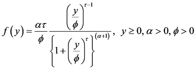 . (2.2.1)
The algorithm for finding the maximum likelihood estimators (MLE) for the parameters of the Burr XII distribution is taken from [12] and this algorithm exploits the link between the three parameter Burr XII distribution and the two parameter Weibull distribution with the latter emerging as the limiting case of the former
The basic two parameter Burr XII distribution with shape parameters  and
and  has the cumulative distribution function
 . (2.2.2)
An scale parameter  is introduced into (2.2.2) by substituting
 , thereby giving the cdf of y as
 . (2.2.3)
Letting  with
with ![]() remaining finite, and comparing with the cdf of Weibull given in Equation (2.1.1), it is seen that the Burr XII distribution emerges as the limiting distribution for the Weibull distribution
remaining finite, and comparing with the cdf of Weibull given in Equation (2.1.1), it is seen that the Burr XII distribution emerges as the limiting distribution for the Weibull distribution
with shape parameter ![]() and scale parameter
and scale parameter ![]()
For a sample of “m” items ![]() from the Burr XII distribution, the log likelihood is given by
from the Burr XII distribution, the log likelihood is given by
![]() (2.2.4)
(2.2.4)
where ![]() and
and ![]()
The main steps of the algorithm are:
Step 1: First, we find the maximum likelihood of the parameters ![]() appearing in (2.1.2) using the Multi parameter Newton Raphson Iterative method yielding the two values
appearing in (2.1.2) using the Multi parameter Newton Raphson Iterative method yielding the two values ![]() and
and![]() . In our case, in estimating the MLE for the parameters of the Weibull in the former section, they have already been obtained.
. In our case, in estimating the MLE for the parameters of the Weibull in the former section, they have already been obtained.
Step 2 Then, we rescale the original data by ![]() so that in implementing the Newton Raphson for determining
so that in implementing the Newton Raphson for determining
the MLEs of the parameters of the Burr XII distribution, the utilized values are the rescaled values ![]()
The argument in [12] leads us to conclude that rescaling the data introduces a large amount of stability into the algorithm. After the parameter estimates have been obtained, the MLE for the Burr XII distribution for the original observations are obtained by undoing the effect of scaling on the estimated values of the parameters.
In the appendix: (1) of [13] , we have obtained the Gradient and the Hessian Matrices for estimating the parameters of the Burr XII distribution through the algorithm stated in [12] .
2.3. Classical Risk Model
Let ![]() denote the surplus process of an insurer as
denote the surplus process of an insurer as
![]() (2.3.1)
(2.3.1)
where ![]() is the initial surplus, c is the rate of premium income per unit time and
is the initial surplus, c is the rate of premium income per unit time and ![]() is the aggregate
is the aggregate
claim process and we have ![]() where
where ![]() is a homogeneous Poisson process with parameter
is a homogeneous Poisson process with parameter![]() ,
, ![]() denotes the amount of the ith claim and
denotes the amount of the ith claim and ![]() is a sequence of iid random variables with distribution function F such that
is a sequence of iid random variables with distribution function F such that ![]() and probability density function f. We denote
and probability density function f. We denote ![]() by
by![]() . Also we have
. Also we have![]() , where
, where ![]() is the security loading factor.
is the security loading factor.
Let ![]() denote the time to ruin from initial surplus u so that
denote the time to ruin from initial surplus u so that
![]() and define
and define ![]() and
and![]() .
. ![]() is known as the ultimate ruin probability whereas
is known as the ultimate ruin probability whereas ![]() is the finite time ruin probability. For a detailed discussion on the Classical Risk model and the probability of ruin refer to [2] [10] [14] [15] .
is the finite time ruin probability. For a detailed discussion on the Classical Risk model and the probability of ruin refer to [2] [10] [14] [15] .
Classical Risk model, despite the fact that it is considered to be the basis of many models in insurance mathematics involves many simplication criterions which make it deviate from the real life situations. For example, the assumptions like the independence between the claim severity and the claim number distributions, the intensity parameter ![]() being independent of time etc are not very consistent with the real scenario observed in the insurance companies. Ruin, in some sense corresponds to the insolvency of an insurance company and hence, the probability of ruin is a very useful tool in long range planning for the use of the insurer’s funds.
being independent of time etc are not very consistent with the real scenario observed in the insurance companies. Ruin, in some sense corresponds to the insolvency of an insurance company and hence, the probability of ruin is a very useful tool in long range planning for the use of the insurer’s funds.
2.4. Pollaczek-Khinchin Formula for the Probability of Ultimate Ruin
As given in [16] , the probability of ultimate ruin satisfies the following integro differential equation
![]() . (2.4.1)
. (2.4.1)
If L is the maximal aggregate loss random variable, then it can be shown that
![]() (2.4.2)
(2.4.2)
where ![]() is the amount of the
is the amount of the ![]() drop of the Surplus process and because the Surplus Process has stationary and independent increments ,
drop of the Surplus process and because the Surplus Process has stationary and independent increments , ![]() is a sequence of independent and identically distributed random variables each with density
is a sequence of independent and identically distributed random variables each with density
![]() . (2.4.3)
. (2.4.3)
And the number of drops K is geometrically distributed with the parameter ![]() (refer to [1] [11]
(refer to [1] [11]
[17] ).
It is evident that ruin never occurs or that the company survives if starting with an initial surplus of u, the maximal aggregate loss random variable L never exceeds u i.e. the probability of ultimate survival is: ![]()
Let ![]() and
and ![]() is the cumulative distribution function
is the cumulative distribution function
of the K-fold convolution of the distribution of Y with itself.
Then the general solution to Equation (2.4.1) is given by (see [1] )
![]() , where
, where![]() . (2.4.4)
. (2.4.4)
Equation (2.4.4) is known as the Pollaczek-Khinchin formula for the Probability of ultimate ruin.
An explicit expression for the probability of ultimate ruin can be derived through the use of the Pollaczek-Khinchin formula for those claim amount distributions whose Laplace transforms have closed form expressions [18] [19] . However, in case of heavy tailed distributions like Weibull, Burr, Log Normal etc, their Laplace transform don’t have a closed form expression and hence, this procedure of obtaining an explicit expression for the probability of ultimate ruin through inversion of the Laplace transform is not applicable. For such cases, the use of the Pollaczek Khinchin formula to obtain an approximation to the Probability of ultimate ruin can be made through Monte Carlo Simulation.
In the subsequent section, we give a brief description to the computation of the approximation to the probability of ultimate ruin from the Pollaczek-Khinchin formula through Monte Carlo simulation. However, one of the main objectives of this paper is to lay down a methodology to simulate observations from the Equilibrium distributions of Burr XII and Weibull and to use these observations to obtain an approximation to the Probability of Ultimate Ruin from the Pollaczek-Khinchin formula. In fact, the simulation from the Equilibrium distribution in case the claim severity is heavy tailed, constitutes one of the main challenges in the application of the above simulation procedure to obtain an approximation to the Probability of ultimate ruin.
In [20] , three methods to simulate the Probability of Ultimate ruin are presented and their asymptotic efficiencies being investigated. What they referred to as Algorithm I, is a crude Monte Carlo method and we shall use this algorithm to obtain ![]() through simulation. To simulate from the equilibrium distribution, they have used a conditional Monte Carlo method, which as indicated by them is not asymptotically efficient in the sense of a criterion mentioned in [21] . Further modifications to this algorithm is suggested in [20] but we restrain from elaborately discussing it and have concentrated on the rejection method to simulate observations from the Equilibrium distributions of Burr XII and Weibull and thereafter, have used these simulated observations to obtained an approximation to
through simulation. To simulate from the equilibrium distribution, they have used a conditional Monte Carlo method, which as indicated by them is not asymptotically efficient in the sense of a criterion mentioned in [21] . Further modifications to this algorithm is suggested in [20] but we restrain from elaborately discussing it and have concentrated on the rejection method to simulate observations from the Equilibrium distributions of Burr XII and Weibull and thereafter, have used these simulated observations to obtained an approximation to ![]() through algorithm I as mentioned in [20] . It needs to be mentioned that the basis of algorithm I is the Pollaczek-Khinchin formula discussed above.
through algorithm I as mentioned in [20] . It needs to be mentioned that the basis of algorithm I is the Pollaczek-Khinchin formula discussed above.
2.4.1. The Algorithm for Obtaining y(u) from Pollaczek-Khinchin Formula through Monte Carlo Simulation (Algorithm I of [20] )
Step 1: Generate ![]() -Geometric
-Geometric ![]()
Step 2: Generate ![]() from the density
from the density ![]() and let
and let
![]()
Step 3: If![]() , then set
, then set ![]() otherwise
otherwise ![]()
Step 4: Repeat steps 1 to 3n (the number of times the simulations is to be carried out) times.
Step 5: Estimate E(z) by
![]()
An approximation to ![]() is given by
is given by ![]()
2.4.2. Rejection Method for Generating Observations from the Equilibrium Distributions of Burr XII and Weibull Distributions
We have used the rejection method for generating random observations from the equilibrium distributions of Burr XII and Weibull distributions. As outlined in [22] , the Rejection method is used when we have a known method to generate from a random variable having density ![]() and we need to generate from an another density
and we need to generate from an another density ![]() such that the known method for
such that the known method for ![]() can be manipulated to generate from the density
can be manipulated to generate from the density![]() .
.
The algorithm for generating observations from ![]() using the rejection method is as follows
using the rejection method is as follows
Step 1 Generate Y having density g.
Step 2: Generate a random number U.
Step 3: If![]() , set
, set![]() , otherwise return to step 1,
, otherwise return to step 1,
where c is a constant such that
![]() for all Y.
for all Y.
Here X can be considered to be a random observation generated from the density ![]()
2.4.3. Equilibrium Distribution
If ![]() is the cumulative distribution function of the claim severity distribution, then the Equilibrium distribution associated with the claim severity has the probability density function given by
is the cumulative distribution function of the claim severity distribution, then the Equilibrium distribution associated with the claim severity has the probability density function given by
![]() . As it can be seen from Equation (2.4.3), it is the density function of the
. As it can be seen from Equation (2.4.3), it is the density function of the ![]() drop
drop
(![]() ) and hence is a vital requirement for the evaluation of the probability of ruin through the Pollaczek-Khinchin formula ( [23] and [24] ).
) and hence is a vital requirement for the evaluation of the probability of ruin through the Pollaczek-Khinchin formula ( [23] and [24] ).
2.4.4. Generating from the Equilibrium Distribution of Burr XII
The density of the Equilibrium distribution of Burr XII is given by
![]() (2.4.5)
(2.4.5)
where ![]()
The inverse transform algorithm (see [22] ) can be used to generate observations from the Burr XII distribution. Hence, ![]() can be the density of the original Burr XII distribution.
can be the density of the original Burr XII distribution.
Therefore,
![]() . (2.4.6)
. (2.4.6)
Our goal is to generate observations from ![]() and for this, we first need to generate observations from the Burr XII distribution and for generating random observations from Burr XII, we shall use the inverse transform algorithm as described below.
and for this, we first need to generate observations from the Burr XII distribution and for generating random observations from Burr XII, we shall use the inverse transform algorithm as described below.
Let U be a random number lying between 0 and 1 and the cumulative distribution function of the Burr XII is given by
![]()
Hence the transform equation is
![]() . (2.4.7)
. (2.4.7)
Solving for y gives
![]() . (2.4.8)
. (2.4.8)
Now, we need to find c such that
![]() i.e.
i.e. ![]()
Let ![]() (say).
(say).
To maximize, ![]() , we proceed as follows
, we proceed as follows
![]() (2.4.9)
(2.4.9)
Therefore, ![]()
Þ Either ![]() or
or ![]()
Now ![]() implies
implies ![]() which is not possible.
which is not possible.
Hence, ![]()
which gives![]() . (2.4.10)
. (2.4.10)
It can be shown that for this value of y, ![]()
Therefore, ![]() where
where![]() . (2.4.11)
. (2.4.11)
Therefore,
![]() . (2.4.12)
. (2.4.12)
Hence the algorithm for generating random observations from the Equilibrium distribution of Burr XII is
Step 1: Generate a random number ![]() and set
and set ![]()
Step 2: Generate a random number ![]()
Step 3: If![]() , where
, where![]() , (k is given by Equation (2.4.11)) then set
, (k is given by Equation (2.4.11)) then set
![]() , otherwise return to step 1.
, otherwise return to step 1.
Here, x can be considered to be a random observation generated from the Equilibrium distribution of Burr XII.
Repeat the above steps as many times as the number of random observations required from the Equilibrium distribution of the Burr XII distribution.
2.4.5. Generating from the Equilibrium Distribution of Weibull
The density of the Equilibrium distribution of Weibull is given by
![]() (2.4.13)
(2.4.13)
Here ![]()
Here unlike the situation in Burr XII distribution, ![]() cannot be the density of the original Weibull distri-
cannot be the density of the original Weibull distri-
bution because in that case ![]() cannot be maximized. Instead, we choose to take
cannot be maximized. Instead, we choose to take ![]() as the density of the exponential distribution with parameter
as the density of the exponential distribution with parameter![]() . It may be noted that if in the pdf of the Weibull dis-
. It may be noted that if in the pdf of the Weibull dis-
tribution given in Equation (2.1.2), we choose the shape parameter ![]() as
as![]() , we get the pdf of the expo-
, we get the pdf of the expo-
nential distribution with parameter ![]() i.e. Weibull with
i.e. Weibull with ![]() is exponential with parameter
is exponential with parameter ![]() (see [25] ).
(see [25] ).
If U is a random number, using inverse transform algorithm it can be shown that an observation generated
from the exponential distribution with parameter ![]() is given by
is given by
![]()
Next, we need to find c such that
![]()
i.e. ![]()
let ![]()
![]() . (2.4.14)
. (2.4.14)
Therefore, ![]() , since
, since ![]()
![]() . (2.4.15)
. (2.4.15)
It can be shown that for this value of y, ![]()
Therefore,![]() (2.4.16)
(2.4.16)
and
![]() . (2.4.17)
. (2.4.17)
And
![]()
Hence the algorithm for generating random observations from the Equilibrium distribution of Weibull is:
Step 1: Generate a random number ![]() and set
and set ![]()
Step 2: Generate a random number ![]() and if
and if ![]() where K is given by Equation (2.4.17), set
where K is given by Equation (2.4.17), set
![]() , Otherwise return to step 1.
, Otherwise return to step 1.
Here X can be considered as a random observation generated from the equilibrium distribution of Weibull and the process is repeated as many times as the number of random observations required to be generated from the equilibrium distribution.
2.4.6. Assessing the Efficiencies of the Simulation Schemes
In assessing the efficiency of our simulation scheme, we have adopted the following procedure.
As given is Equation (2.4.2),
If L is the maximal aggregate loss random variable, then it can be shown that
![]()
where ![]() is the amount of the
is the amount of the ![]() drop of the Surplus process and because the Surplus Process has stationary and independent increments,
drop of the Surplus process and because the Surplus Process has stationary and independent increments, ![]() is a sequence of independent and identically distributed random variables each with density
is a sequence of independent and identically distributed random variables each with density
![]()
And the number of drops K is geometrically distributed with the parameter ![]()
Also as shown in [16] ,
![]() . (2.4.18)
. (2.4.18)
Using our simulation schemes, we have simulated 20 values of L for each of the cases, when the claim severity is Burr XII and when the claim severity is Weibull. The mean of L obtained through simulation is compared with ![]() to get an idea on the efficiency of the simulation scheme.
to get an idea on the efficiency of the simulation scheme.
2.5. Convolution of the Burr XII Distribution and the Weibull Distributions
In this section, we have attempted to carry out the convolution of the Burr XII distribution with itself and the convolution of the Weibull distribution with itself and illustrated their applications in computing the Probability function of the number of claims until ruin in case of zero initial surpluses. The convolution of the Burr XII distribution and the Weibull distribution can be carried out only numerically. It can be noted that evaluation of the ![]() convolution would require
convolution would require ![]() convolution as input, for example evaluation of the third convolution would require second convolution as input and the evaluation of the fourth convolution would require the third convolution as input and so on, resulting in a very complex situation, where one has to deal with a number of nested integrals.
convolution as input, for example evaluation of the third convolution would require second convolution as input and the evaluation of the fourth convolution would require the third convolution as input and so on, resulting in a very complex situation, where one has to deal with a number of nested integrals.
Here we have obtained the convolution of the Burr XII distribution and Weibull up to the fourth order in the form of integrals which were evaluated numerically using R program.
2.5.1. Convolution of the Burr XII Distribution
First convolution of the Burr distribution is its pdf itself.
1) Second Convolution of the Burr Distribution
The second convolution of the Burr XII distribution is the distribution of
![]() , where
, where ![]() and
and ![]() are both independent and each distributed as Burr XII.
are both independent and each distributed as Burr XII.
The pdf of Z is given by
![]() (2.5.1)
(2.5.1)
It is not possible to find an explicit expression for it and it has to be computed only numerically.
2) Third Convolution of the Burr distribution
The third convolution of the Burr XII distribution is the pdf of
![]() , where
, where ![]() and
and ![]() are all independent and each distributed as Burr XII
are all independent and each distributed as Burr XII
The pdf of ![]() is given by
is given by
![]() . (2.5.2)
. (2.5.2)
Similarly, the nth convolution of the Burr XII distribution is given by
![]() . (2.5.3)
. (2.5.3)
It is to be noted that in determining the ![]() convolution, the
convolution, the ![]() convolution is taken as input.
convolution is taken as input.
2.5.2. Convolution of the Weibull Distribution
First convolution of the Weibull is its pdf itself.
1) Second Convolution of Weibull
The second convolution of Weibull is the distribution of
![]() , where
, where ![]() and
and ![]() are both independent and each distributed as Weibull.
are both independent and each distributed as Weibull.
The pdf of Z is given by
![]() , where
, where ![]() is the pdf of the Weibull distribution.
is the pdf of the Weibull distribution.
![]() . (2.5.4)
. (2.5.4)
As in the case of Burr XII, this also can only be evaluated numerically.
Likewise, the third and the higher order convolutions of Weibull can be defined and as in the case of Burr XII, they can be evaluated only numerically and as stated earlier, the ![]() convolution would take the
convolution would take the ![]() convolution as one of its inputs.
convolution as one of its inputs.
The distribution of the number of claims until ruin has been studied by a number of authors over the year. Reference [26] derives the Laplace transformation of the probability function of the number of claims until ruin in the classical risk model. Reference [27] uses probabilistic arguments to find an expression for the density of the time to ruin in the classical Risk model and this approach is further adopted to obtain an expression for the joint density of the time to ruin and the number of claims until ruin in [28] He derived the marginal distribution of the number of claims until ruin from this joint density.
In this paper, we have used the results derived in [28] to find the probability function of the number of claims until ruin in case of Burr XII distribution and Weibull distribution considering zero initial surplus for just![]() ,
, ![]() and
and ![]() (i.e. the probability function for 2, 3 and 4 number of claims until ruin are computed) ,our main intention being to illustrate the complexity involved in obtaining the convolution of these distributions.
(i.e. the probability function for 2, 3 and 4 number of claims until ruin are computed) ,our main intention being to illustrate the complexity involved in obtaining the convolution of these distributions.
We state the results from [28] which are used to determine the probability of the number of claims until ruin.
Probability function for the number of claims until ruin for zero initial surplus is given by
![]() and (2.5.5)
and (2.5.5)
for ![]()
![]() (2.5.6)
(2.5.6)
where ![]() denotes the probability that m number of claims occurs until ruin when the initial surplus is zero.
denotes the probability that m number of claims occurs until ruin when the initial surplus is zero.
Here, we note that in obtaining![]() , we require the convolution of the
, we require the convolution of the ![]() order of the underlying claim severity distribution.
order of the underlying claim severity distribution.
Inserting ![]() and 4, in Equation (2.5.6)
and 4, in Equation (2.5.6)
we have ![]() (2.5.7)
(2.5.7)
![]() (2.5.8)
(2.5.8)
and
![]() . (2.5.9)
. (2.5.9)
3. Results and Discussions
Data: Our data is a set of 160,000 claim amounts spread over a period of 6 months i.e. April, 2013 to September, 2013 from a General Insurance company from its motor insurance portfolio covering all its branches in India. No adjustment was made for inflation for the time horizon is narrow. It needs to be mentioned that the data is utilized more for the illustration of the various methodologies rather than for the extraction of any concrete meaningful conclusion.
Summary statistics of the data as shown in Table 1 reveal the existence of high coefficient of skewness which suggests that a highly skewed right tailed distribution such as the Burr XII or Weibull can be a probable candidate for modeling this data. The histogram of the data plotted in Figure 1 and the empirical probability density function plotted in Figure 2 show the same trend. These figures too indicate a high degree of skewness towards
![]()
Table 1. Summary statistics for the insurance claim data.
![]()
Figure 1. Histogram of the observed claim data on motor insurance.
![]()
Figure 2. Estimate of the probability density function for the claim data on motor insurance.
the right, which in a way, justifies the use of these heavy tailed distributions for modeling our data.
For finding the maximum likelihood estimators for the parameters of the Weibull distribution, the use has been made of the Multi parameter Newton Raphson method. Table 2 shows the estimates of the parameters thus obtained for the Weibull distribution. The assessment of the fit of the Weibull distribution was done through some graphical displays and then through the computation of some EDF statistics namely the Anderson Darling Statistics and the Cramer Von Mises Statistics [30] . The histogram for a set of data simulated from the Weibull distribution with the values of the parameters, as those of the estimated values (Figure 3) reveals that the Weibull distribution can be a potential model for our data and the same conclusion is validated from the QQ plot for the Weibull distribution (Figure 4) with the less than extreme deviation of the QQ plot from the straight line passing through the origin. However, the EDF statistics indicate the lack of fit since the values of these statistics for our data were found to be significantly high and their p-values computed through Monte Carlo simulation [22] were considerably low. In finding the MLE for the parameters of the Burr XII distribution, the use of the algorithm mentioned in [12] has been made. The log likelihood got maximized at the 30th iteration thereby giving the estimated values of the parameters as shown in Table 3. In case of the assessment for Burr XII fit, initial assessment was done through some graphical displays. Figure 5 shows the histogram for a set of data simulated from the Burr XII distribution with the values of the parameters as estimated using the algorithm. This histogram has some resemblance with the histogram for the observed data as shown in Figure 1. The QQ plot forth Burr XII distribution displayed in Figure 6 indicates moderate deviation from the straight line passing through the origin. Table 3 shows the values of the Anderson Darling and the Cramer Von statistics for testing the goodness of fit for the Burr XII distribution along with their p-values obtained through the Monte-Carlo simulation based on 100 iterations [22] .
In making a comparative assessment of the fit as to judge which of the two distributions is providing a better fit to the data, values of the log-likelihood indicate that compared to Weibull, Burr XII is modeling the data in a better way since the log-likelihood for the sample in case of Burr XII is more than that for Weibull (Log-like- lihood for the sample under the fitted Weibull was found to be −1726599 and that for the fitted Burr XII was found to be −162475.8).
Hence, we have little evidence to believe that either the Burr XII distribution or Weibull distribution adequately describes the claim data. In the subsequent sections, we have used this fitted Weibull distribution mainly with the objective of depicting the computational methodologies associated with the Weibull distribution in obtaining some of the important Actuarial Quantities viz the Probability of ultimate ruin and probability function for the number of claims until ruin. However, the fitted Burr XII distribution was excluded from being used in the subsequent computational methodologies for the current limitations encountered in our computing schemes, with the occurrence of numerical error being indispensable, it leads to some absurd results which were difficult to interprete in the normal framework. Instead, an illustrative Burr XII distribution was used for displaying the complexity associated in determining these actuarial quantities in case of Burr XII claim severity distribution.
One of the main objectives of this paper was to lay down methodologies to simulate from the equilibrium distributions of Weibull and Burr XII distributions and as indicated earlier, these simulations constitute a vital component for the evaluation of the probability of ultimate ruin through the Pollaczek-Khinchin formula. Table 4 shows a sample of 5 observations and another sample of 10 observations drawn from the Equilibrium distribution
![]()
Table 2. Parameter estimates for the Weibull distribution obtained through the multi parameter Newton Raphson and the value of the EDF statistics along with their p-values indicated in parentheses.
![]()
Table 3. Parameter estimates for the Burr XII distribution obtained through the Watkin algorithm and the value of the EDF statistics along with their p-values indicated in parentheses.
![]()
Table 4. Samples of random observations drawn from the equilibrium distribution corresponding to the illustrative Burr XII with ![]() and
and![]() .
.
![]()
Figure 3. Histogram for a data set simulated from the Weibull distribution with ![]() and
and![]() .
.
![]()
Figure 4. QQ Plot between the empirical quantiles estimated from the motor insurance data and the theoretical quantiles for the Weibull distribution with ![]() and
and![]() .
.
of Weibull whereas Table 5 shows a sample of 5 observations and a sample of 10 observations drawn from the Equilibrium distribution of Burr XII. Sample standard deviation of the sample of size n = 10 drawn from the Equilibrium distributions of Burr XII was found to be 54,409.1 whereas that for the sample drawn from the equilibrium distribution of Weibull, it was found to be 7983.253. These values indicate a high degree of heterogeneity in the sample of random observations drawn from the corresponding equilibrium distributions. However,
![]()
Figure 5. Histogram for a data set simulated from the Burr XII distribution with ![]() and
and![]() .
.
![]()
Figure 6. QQ Plot between the empirical quantiles estimated from the motor insurance data and the theoretical quantiles for the burr XII distribution with ![]() and
and![]() .
.
![]()
Table 5. Samples of random observations drawn from the equilibrium distribution corresponding to the fitted Weibull with ![]() and
and![]() .
.
to appraise the efficiencies of the simulation schemes, the direct expressions for the mean and variance (theoretical) of these equilibrium distributions were not available and therefore, we have used an indirect way to assess the efficiencies of these schemes.
The maximal aggregate loss random variable is related to the simulated observations by Equation (2.4.2) and a direct expression for the mean of L is given by Equation (2.4.18). Hence a comparison of the mean of L obtained through our simulation schemes with that of ![]() gives some idea on the efficiencies of these schemes. For the illustrative Burr XII distribution, Table 6 shows the 20 values of L. The mean of L computed on the basis of these 20 simulations was found to be 51,153.72 whereas the theoretical mean of L in case of the illustrative Burr XII distribution, computed by Equation (2.4.18) was found to be 327,164.3 This lack of consistency between the simulated value and the theoretical value is attributed to the fact that simulation is always an approximation and can never be that close to the actual value. It needs noting that three simulation schemes are behind the calculation of the simulated mean of L and thereby, each leading to some inconsistency in the match with the theoretical value. Also, we carried out only twenty simulations and it can be expected that a larger number of simulations would have added some more efficiency to the simulated mean. However, it needs exploring to insert some modifications into the simulation scheme to improve its efficiency. Similarly in case of Weibull distribution, Table 7 shows the 20 simulations carried out to obtained the simulated mean of L and even in this case, there is inconsistency between the simulated and the theoretical mean of L for the theoretical mean of L in case of our fitted Weibull is found to be 58,576.9 whereas the simulated mean has come out to be 10,225.57. The justification put forward for the lack of consistency in case of Burr XII is also applicable in explaining the lack of consistency between the theoretical mean and the simulated mean of the equilibrium distribution corresponding to Weibull.
gives some idea on the efficiencies of these schemes. For the illustrative Burr XII distribution, Table 6 shows the 20 values of L. The mean of L computed on the basis of these 20 simulations was found to be 51,153.72 whereas the theoretical mean of L in case of the illustrative Burr XII distribution, computed by Equation (2.4.18) was found to be 327,164.3 This lack of consistency between the simulated value and the theoretical value is attributed to the fact that simulation is always an approximation and can never be that close to the actual value. It needs noting that three simulation schemes are behind the calculation of the simulated mean of L and thereby, each leading to some inconsistency in the match with the theoretical value. Also, we carried out only twenty simulations and it can be expected that a larger number of simulations would have added some more efficiency to the simulated mean. However, it needs exploring to insert some modifications into the simulation scheme to improve its efficiency. Similarly in case of Weibull distribution, Table 7 shows the 20 simulations carried out to obtained the simulated mean of L and even in this case, there is inconsistency between the simulated and the theoretical mean of L for the theoretical mean of L in case of our fitted Weibull is found to be 58,576.9 whereas the simulated mean has come out to be 10,225.57. The justification put forward for the lack of consistency in case of Burr XII is also applicable in explaining the lack of consistency between the theoretical mean and the simulated mean of the equilibrium distribution corresponding to Weibull.
![]()
Table 6. Simulation for obtaining the mean of the maximal aggregate loss random variable L for the illustrative Burr XII distribution with ![]() and
and![]() .
.
Therefore, the simulated mean of L based on 20 simulations is (101,374.6 + 139,696.3 + ∙∙∙ +412,416.2)/20 = 51,153.72.
![]()
Table 7. Simulation for obtaining the mean of the maximal aggregate loss random variable L for the fitted Weibull distribution with ![]() and
and![]() .
.
Therefore, the simulated mean of L based on 20 simulations is (54,042.1 + 17,896.88+ ∙∙∙ +24,710.59)/20 = 10,225.57.
The algorithm for the evaluation of the probability of ultimate ruin through the Pollaczek Khinchin formula as described in section (2.4.1) shows how the simulated observations are to be used in evaluating the Probability of ultimate ruin in case of Weibull and Burr XII distributed claim severity. Table 8 shows the probability of ultimate ruin obtained through the Pollaczek-Khinchin formula for the illustrative Burr distribution with a security loading of 0.3 whereas Table 9 shows the corresponding values for the fitted Weibull distribution. In both the cases, the Probability of ultimate ruin was found to be a decreasing function of the initial surpluses and this is expected, as larger initial surpluses should diminish the chance of ruin (if any) for the insurance company. The probability of ultimate ruin for the Burr XII distribution was computed through two numerical algorithms namely the stable recursive algorithm and the method of product integration in [13] . It is observed that there is deviation in the values obtained through these two algorithms and the Pollaczek-Khinchin formula. Although the lack of efficiency in the simulation schemes can be one of the causes for this deviation, yet there is no standard baseline method in terms of which the most efficient numerical computation method for the probability of ultimate ruin in case of Burr XII claim severity can be established.
Computation of the convolutions of a distribution with itself is very challenging, specially, when the distribution does not have a closed form expression for its Laplace transform (Moment generating function) and since neither Weibull nor Burr XII has closed form Laplace transform, their convolutions can be determined only
![]()
Table 8. Ultimate ruin probabilities for the burr XII distribution with ![]() and
and ![]() obtained through Pollaczek-Khinchin formula based on 10,000 simulations.
obtained through Pollaczek-Khinchin formula based on 10,000 simulations.
![]()
Table 9. Ultimate ruin probabilities for the fitted Weibull distribution with ![]() and
and ![]() obtained through Pollaczek-Khinchin formula based on 10,000 simulations.
obtained through Pollaczek-Khinchin formula based on 10,000 simulations.
numerically. Table 10 shows the convolution of our fitted Burr XII distribution upto the fourth order and Table 11 shows the corresponding values for the fitted Weibull. These convolutions were evaluated at a number of points solely for the sake of illustration. It may be noted that in evaluating these convolutions, numerical integrations were used and a number of nested integrals were evaluated to get the final output. Hence, this might led to the accumulation of a considerable error. Another issue associated with this convolution is the high execution time for example, in evaluating![]() ,say, for Weibull, three nested integrals were to be computed simultaneously, one for
,say, for Weibull, three nested integrals were to be computed simultaneously, one for ![]() and using this as an input, another numerical integral
and using this as an input, another numerical integral ![]() was computed. Again, since we are using the Simpson’s 1/3 rd rule for numerical integration, for computing
was computed. Again, since we are using the Simpson’s 1/3 rd rule for numerical integration, for computing![]() ,
, ![]() needs to be computed at a considerable large number of points (for it appears in the integrand for
needs to be computed at a considerable large number of points (for it appears in the integrand for![]() and if we require some extra accuracy by limiting the interval of discretization at
and if we require some extra accuracy by limiting the interval of discretization at![]() ., the computational time threatens to be very high. Moreover with this fixed level of discretization, number of intervals (hence the number of computations) increases largely with an increase in the value of z (the point where
., the computational time threatens to be very high. Moreover with this fixed level of discretization, number of intervals (hence the number of computations) increases largely with an increase in the value of z (the point where ![]() is to be computed). This execution procedure takes hours, even at times, exceeding 6 hours unless we deliberately fixed the number of intervals at a lower level (say 100) for each of these numerical integrations, allowing variability in h, at the
is to be computed). This execution procedure takes hours, even at times, exceeding 6 hours unless we deliberately fixed the number of intervals at a lower level (say 100) for each of these numerical integrations, allowing variability in h, at the
![]()
Table 10. First four convolutions of the Burr XII distribution with ![]() and
and ![]() determined at some illustrative points.
determined at some illustrative points.
![]()
Table 11. First four convolutions of the fitted Weibull distribution with ![]() and
and ![]() determined at some illustrative points.
determined at some illustrative points.
cost of reducing some accuracy in the values obtained through these numerical integrations.
The computation of the probability function of the number of claims until ruin requires the computation of the convolution of the underlying claim severity distribution, for example, the computation of the probability function for 3 number of claims until ruin would require second convolution as an input, 4 number of claims until ruin would require third convolution and so on. Table 12 shows the probability for 2, 3 and 4 number of claims until ruin for the illustrative Burr XII distribution whereas Table 13 shows the corresponding values for the Weibull distribution. It needs to be noted that though, Table 10 gives the convolution of the fitted Burr XII distribution, Table 12 was constructed for the illustrative Burr XII distribution whose convolutions were not displayed separately. Numerical error might have affected the results in a way that no proper interpretation within the practical frame work is possible. The result for the Burr XII distribution are somewhat consistent with reality for the values of these probabilities were marginally low and this is interpretable in the practical situation for the chance of ruin should be very low for such small number of claims.
We give some insight into the numerical integration underlying the computation of ![]() and similar explanation accounts for
and similar explanation accounts for ![]() and
and![]() . The main difficulty lies in the fact that in their computations, we are handing double integrals and those too involving convolutions and furthermore, the outer integral needs to be evaluated at a range extending to infinity.
. The main difficulty lies in the fact that in their computations, we are handing double integrals and those too involving convolutions and furthermore, the outer integral needs to be evaluated at a range extending to infinity.
From Equation (2.5.9), we have ![]()
1) We have first evaluated ![]() as a function of t. Let this function be denoted as
as a function of t. Let this function be denoted as![]() .
.
Here we have used the function for 3rd convolution of Burr XII as required in ![]()
2) Now consider the integrand ![]() of
of ![]() which is to be integrated with
which is to be integrated with
respect to t in the interval ![]() and this integrand can be denoted as an another function of t, say
and this integrand can be denoted as an another function of t, say
![]() . For the assumed values of the parameters of Burr XII, this function was computed in a
. For the assumed values of the parameters of Burr XII, this function was computed in a
number of intervals of values for t and was found to have significant value only in the interval [1e−06, 22], its value being zero beyond it. The final value was obtained by numerical integration of ![]() using Simpson’s 1/3rd rule in the interval [1e−06, 22].
using Simpson’s 1/3rd rule in the interval [1e−06, 22].
Interestingly, it may be noted from Equation (2.5.6), that to find the probability function of “m” number of claims until ruin (in case of zero initial surplus), it is required to use the ![]() convolution of the underlying claim severity distribution. Hence, it can be sensed that there is huge complexity involved in determining this function for
convolution of the underlying claim severity distribution. Hence, it can be sensed that there is huge complexity involved in determining this function for![]() . As a practical consideration, it might be realized that this probability function is useful only when it can be determined for “m” very large because it is sensible to assume that ruin could occur only when “m” is very large.
. As a practical consideration, it might be realized that this probability function is useful only when it can be determined for “m” very large because it is sensible to assume that ruin could occur only when “m” is very large.
4. Limitations
This paper has chance to provide themes for further exploration if means are devised to eliminate the following limitations.
1) Neither of the distribution was found to qualify the goodness of fit tests, as judged, from the EDF statistics, though we proceeded with the use of the estimated values of the parameters of the fitted Weibull distribution as input for the computational methodologies, targeted at the evaluation of the actuarial quantities under consideration.
2) The fitted Burr XII distribution had to be excluded from being used as an input for the computational methodologies for it led to some inconsistent results. It needs further scrutiny to identify the cause for these inconsistencies.
3) The simulation schemes need to be further improved for the values of the probability of ultimate ruin for the Burr XII distribution, it yielded are inconsistent to the values computed earlier [13] .
4) To avoid the complexity of having to evaluate a number of nested integrals numerically, we had to remain content with the evaluation of just the lower order convolution of these distributions, which, in turn, enabled us to compute the probability function for the number of claims until ruin, for a lower ranking whose significance to reality is not as important as the function, computed for a higher ranking of the order at which the claims arrive.
5. Conclusions and Further Extensions
Modeling of the insurance data through these two heavy tailed distributions is quite a challenge in the realm of statistical computational theory and considering the fact, that highly skewed data which can be adequately modeled only through heavy tailed distributions, occurs frequently in the domain of General insurance, our work might be useful for insurance practitioners concerned with statistical modeling in Risk analysis.
Methodologies suggested for the simulation from the Equilibrium distributions of Burr XII and Weibull were reasonably efficient and when applied to the algorithms for the evaluation of the probability of ultimate ruin through simulation using the Pollaczek-Khinchin formula, they led to fairly good approximations to the probability of ultimate ruin and these approximations were also consistent with practical rationalism. However, further exploration is needed to improve these simulation schemes, for example, by implementing conditional Monte Carlo algorithms and by using some properties of the family of the sub-exponential distributions (of which Weibull and Burr XII are members) to improve the algorithms.
The paper has made an attempt to address the complex issue of evaluating the convolution of the Weibull and the Burr XII distributions. Further investigation is needed to identify if any method other than numerical integration exists for the evaluation of the convolution of these heavy tailed distributions. Control of error in evaluating these numerical integrals, reduction in the execution time etc. can be the themes for further probe. Further extension of this work can also be directed towards the evaluation of the convolutions of higher order for they owe much relevance to the assessment of the chances of ruin (insolvency) for the insurance company.