Comparisons between Isotropic and Anisotropic TV Regularizations in Inverse Acoustic Scattering ()
1. Introduction
Inverse acoustic scattering problem is to get the refractive index from measurements of the scattered field or its far field pattern data. It has wide applications in many aspects such as radar, sonar, geophysical exploration, medical CT imaging and nondestructive testing [1] .
Inverse acoustic scattering problem is typically non-linear and ill-posedness. To be precise, the small disturbance of the measurement data could cause severe error in the inversion results. For nonlinearity, the most common way is to adopt linear or optimization method. The regularization method can approximate the ill-posed problem to the well-posed problem to estimate the refractive index distribution. Therefore, iterative regularization method is a typical way to deal with such problems. For example, simplified Newton method [2] , modified gradient method [3] , quasi-Newton method [4] , Gauss-Newton method [5] [6] . In addition, other research results on this issue include: Dual-space method [7] , linear sampling method (LSM) [8] [9] structure recognition function
, which is the solution of the far-field equation
, factorization method
[10] is solved by
in place of the far field equations, multiple
signal classification (MUSIC) [11] [12] constructs a non-iterative solution function, level set method [13] is to determine the regional boundary method.
In this article, we use the isotropic and anisotropic TV regularizations to overcome the ill-posed of inverse acoustic scattering, and the split Bregman algorithm to overcome the non-differentiability of the reconstruction problem and accelerate the inversion process. Finally, the numerical experiment is carried out to verify.
2. Forward Problem and Inverse Scattering Problem
For a given time harmonic incident wave
, the mathematical model of its propagation in inhomogeneous medium can be given by the following Helmholtz equation
(1)
Here,
is the wavenumber, the refractive index function n
is the total field where
represents the scatter field. To ensure the uniqueness of the solution, we require Sommerfeld radiation condition
(2)
uniformly in all directions
. The forward problem is to derive a solution using the Equations ((1), (2)). The forward problem is governed by the following Lippmann-Schwinger equations [1] .
(3)
Here,
is the fundamental solution of the Helmholtz equation i.e.
where
denotes the zero-th order Hankel function of the first kind. Note that for the sake of solving, we assume that the contrast
is satisfied
and
in this article and
is a bound domain where contain the support of the contrast q. For simplicity, we assume that the volume potential V is given by
(4)
so (3) can be described as the following equation
(5)
Hence,
and
.
The forward operator F is defined via:
(6)
The problem of Inverse acoustic scattering can be recast contrast q by the measured data of (6). But, it is well known that (6) is nonlinear about q, which may cause additional complexity in reconstruction methods, so we consider linearizing the above equation. Given the known fixed value q0, we linearize the forward operator F with Taylor polynomial at q0 as the following equation
(7)
where
is measured scattered fields at q0,
is Fréhet derivative of
. For the purpose of computerized reconstruction, we discretize the domain D as
, where
is a rectangle element, then
can be considered as a constant
, q can be approximated by the vector
. We consider minimization of the discretized functional
(8)
Here,
is the jacobian matrix of
,
,
,where
,
represents the number of transmitters, receivers on
. Noting that the measurement data
may have some error due to perturbed measurements or errors, Intuitively, the problem of inverse acoustic scattering can be recast into the following least square error problem to better approximations of the exact solution.
(9)
where
is the searched-for exact contrast,
,
. However, the solution (9) is a complex valued function, so it is difficult to use regularization methods. Thus, we convert a complex-valued functional (9) to a real-valued functional (10) as following
(10)
Here,
,
,
. However, (10) solely minimizing the discrepancy
causes numerical instabilities. Thus, we incorporate a-priori information about the solution to avoid instable results. The most commonly used regularization method is Tikhonov regularization (TR), which is to solve
(11)
with a positive regularization parameter
. However, it has an excessively smooth effect on the solution, which will blur the edge of the reconstructed image. To preserve the shape, we use the isotropic TV
(12)
and anisotropic TV method
(13)
with respectively the first-order difference operators along the x and y directions of
. However, (12) is non-differentiability. So, we use the Split Bregman algorithm to solve the non-differentiability problem, i.e. by introducing new variable
, (12) needs to be converted to minimization problem:
(14)
The minimization of subproblems in (14) can be separated into the minimization of three simple subproblems
and
. Therefore, the following split bregman iteration stages are proposed:
(15)
The (13) is non-differentiability. Similarly, (13) needs to be converted to
(16)
(17)
(18)
(19)
(20)
The first-order optimality condition of (16) is
(21)
The minimization of ((17), (18)) can be found by the soft threshold formula
(22)
Here,
and
are respectively the k-th element of
and
,
is the soft-thresholding operator defined as
(23)
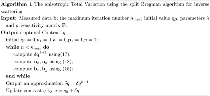
where
is the sign function. We summarize the above procedures as the following algorithm in the form of pseudocode.
3. Numerical Experiments
To validate the proposed method, we demonstrate the reconstruction quality of isotropic TV, anisotropic TV, and Tikhonov regularization methods using some synthetic data. Firstly, we solve the forward problem (3) using the Integral equation to obtain the near field of
as measured data.
All tests were conducted on an Intel Core i7 3.40 GHz CPU and 16 GB of RAM. To avoid “inverse crime,” the discrete computational region of the grid in the forward problem is finer than that in the inverse problem. We show the test set for synthetic data in Figures 1(a)-(f). Here, we choose the domain D as
, wavenumber
and 35 transmitters, receivers on
. we add 1% random noise to measured data for test the stability of method.
In Figure 1, we depict the test set of synthetic data. We apply Tikhonov
regularization, isotropic TV and anisotropic TV methods, respectively, to carry out the numerical simulation. The parameters of the three methods are set to be optimal empirically. It can be seen from Figure 2 that the location of isotropic TV and anisotropic TV reconstruction is more accurate, the shape is closer, and the reconstruction effect is better than the usual Tikhonov regularization (TR) reconstruction.
![]()
Figure 2. The first row (a)-(f) shows that the inversion result of Tikhonov regularization method; the second row (g)-(l) shows the that the inversion result of isotropic TV method; the Third row (m)-(r) shows the that the inversion result of anisotropic TV method.
There are several observations from the two figures. Firstly, all three regularization methods can well capture the main feature of the inner object, including position and shape. From Figures 2(a)-(f) shows that using SB to solve the Tikhonov regularization problem; from Figures 2(g)-(l) show that the images reconstructed by isotropic TV have an obvious ladder effect; from Figures 2(m)-(r) shows that using split Bregman to solve the anisotropic TV regularization problem can obtain an accurate image. The edges of the reconstructed images using the anisotropic TV distort along the coordinate axes.
The numerical experiment shows that the effect of method isotropic and anisotropic TV regularization in inverse acoustic scattering reconstructions is better sharpen the edges and is more robust against data noise than that of method Tikhonov regularization. But, in the anisotropic numerical simulation, the inversion image is distorted along the edge of the coordinate axis alignment, which indicates that there is a large geometric distortion. In order to simplify the operation process and save the running time, we apply the split Bregman algorithm to inverse acoustic scattering problem.
4. Conclusion and Future Work
In this article, we use isotropic TV and anisotropic TV regularization by the split Bergeman method to solve the inverse acoustic scattering problem. These two methods were compared with the Tikhonov method. The simulation results of the measured data show that the isotropic TV regularization can cause a staircase effect; the anisotropic regularization can cause geometric distortion along the coordinate axis. However, these two methods can well preserve boundaries more than Tikhonov regularization. In future work, we will focus on a method that can avoid the distortions along the coordinate axis and does not depend on the selection of regularization parameters.
Acknowledgements
The author would like to thank editor and referees for their valuable advice for the improvement of this article.