Open Journal of Fluid Dynamics
Vol.2 No.3(2012), Article ID:22533,21 pages DOI:10.4236/ojfd.2012.23008
Comparative Analysis of Velocity Decomposition Methods for Internal Combustion Engines
1Department of Aerospace Engineering and Mechanics, The University of Alabama, Tuscaloosa, USA
2Department of Mechanical Engineering, The University of Alabama, Tuscaloosa, USA
Email: solcmen@eng.ua.edu
Received May 25, 2012; revised June 29, 2012; accepted July 25, 2012
Keywords: Proper-Orthogonal Decomposition; Wavelet Decomposition; Principal Component Analysis; LDV; Signal Processing
ABSTRACT
Different signal processing technique performances are compared to each other with regard to separating the mean and fluctuating velocity components of a simulated one-dimensional unsteady velocity signal comparable to signals observed in internal combustion engines. A simulation signal with known mean and fluctuating components was generated using experimental data and generic turbulence spectral information. The simulation signal was generated based on observations on the measured velocity data obtained using LDV in a motored Briggs-and-Stratton engine at about 600 RPM. Experimental data was used as a guide to shape the simulated signal mean velocity variation; fluctuating velocity variations with specified spectrum and standard deviation was used to mimic the turbulence. Cyclic variations were added both to the mean and the fluctuating velocity signals to simulate prescribed cyclic variations. The simulated signal was introduced as input to the following algorithms: ensemble averaging; high-pass filtering; Proper-Orthogonal Decomposition (POD); Wavelet Decomposition (WD) and Wavelet Decomposition/Principal Component Analysis (WD/PCA). The results were analyzed to determine the best method in correctly separating the mean and the fluctuating velocity information, indicating that the WD/PCA performs better compared to other techniques.
1. Introduction
Understanding the nature of turbulence in internal combustion engines is important in studying the underlying mechanisms between turbulence and related phenomena, such as noise generation or lean/clean combustion [1]. Combustion quality depends on the turbulent mixing of fuel and air; turbulence defines the flame speed, burning temperature and the emission of pollutants from combustion processes. Much research has been undertaken to study the in-cylinder flow fields using many different experimental techniques [2], including hotwire anemometry [3], particle tracking velocimetry (PTV) [4-7], particle image velocimetry (PIV) [7-9] and LDV [10-18]. Among these techniques, LDV has been widely used since LDV can be easily adapted to study flow fields within hard to reach geometries such as the valve exit flow or, the flow inside complex bowl-piston configurations [19].
Literature survey indicates that previous research in studying the in-cylinder flow fields is mainly focused on analyzing the data collected in various types of engines using various methods. Erdil et al. [3] used a Ricardo E6/T variable compression engine under motored conditions at 1500 and 2000 RPM and obtained data using hot-wire anemometry for various engine configurations. Data were analyzed using a turbulence filter, ensemble averaging and POD techniques. Roudnitzky et al. [20] applied POD on 2-D time-resolved PIV data obtained in a single transparent cylinder at 1200 RPM to determine the mean component, coherent structures and random Gaussian fluctuations. Fogleman et al. [21] applied the POD technique to datasets obtained in internal combustion engines to emphasize the tumble breakdown instability.
Sullivan et al. [22] used ensemble averaging, highpass filtering and the Wavelet Decomposition in a comparative fashion to analyze the characteristics of turbulence in an L-Head research engine using LDV data obtained at 900 RPM. Their analysis showed that there were no major differences between the mean velocity values plotted as velocity vs. crank-angle profiles, but the power spectral density plots showed considerable difference at frequencies higher than 10 Hz in the range of 0 - 100 Hz. The turbulence energy calculated by the ensemble-averaging technique was about twice the one calculated using high-pass filtering and WD techniques. Ancimer et al. [23] proposed a WD based noise filtering technique to remove the cyclic variations that can occur in the mean velocity to separate the turbulence and the mean velocity variations. Park et al. [18] report LDV measurements made under motored conditions at 1000 RPM in a single cylinder of a V6 3.1 L optical engine, and analysis made using continuous and discrete WD in addition to ensemble averaging and high-pass filtering techniques.
Söderberg et al. [24] discussed the correlation between the heat release and turbulence measurements obtained near the spark plug by a two-component LDV system on a four valve spark ignition engine using WD technique. Measurements were made in a single-cylinder version of a Volvo engine under skip-fired conditions at about 1500 RPM using five different camshafts. Results indicate that combustion rate increases with increased high turbulence rate and results do not change with the use of different wavelet functions. Sen et al. [25] measured the pressure variation in a four-stroke, single-cylinder Aprilia/Rotax spark ignition engine under six different loading conditions to determine the maximum pressure variation in each cycle. The maximum pressure values obtained were then analyzed using Morlet wavelets to determine the periodicity in the signals. The signals were shown to become turbulent at lower cycle counts with increased torque loading. Zhang et al. [26] discuss the difficulties involved in describing turbulence by conventional methods and use an RI-spline-6 wavelet to define the unsteady turbulence intensity using data obtained in a constantvolume cylindrical vessel equipped with optical access to measure the unburned flow velocity using the LDV technique and the flame speed. They further study the effect of the turbulence intensity on the turbulent burning velocity.
A brief summary of the previous research given with selected references and the references included in these publications indicate that ensemble averaging; high-pass filtering; Proper-Orthogonal Decomposition; and Wavelet Decomposition techniques are commonly used in previous research in comparison to each other without the exact knowledge of the performance of the technique in determining the turbulence. In the present work an unsteady signal generated as sum of the mean and fluctuating parts with known statistics is used to compare different analysis techniques and evaluate the performance of these methods. The signal was generated based on the single component velocity data obtained in a BriggsStratton engine using an LDV probe.
In the following sections first the research outline is given, experimental data obtained in a Briggs-and-Stratton engine is briefly described. Section 2 discusses the simulated signal. Section 3 is devoted to describing the analysis methods. Comparison of the performance of analysis methods is given in Section 4, and conclusions derived from the present work are given in Section 5.
1.1. Research Outline
In the current research a simulated signal representing the velocity signal of an internal combustion engine was used to determine the performance of existing methods in calculating the mean and the fluctuating variations of this signal in time. Research was focused on determining the effects of signal duration and signal amplitude on the performance of the methods.
Simulation signal with prescribed mean and fluctuating variations in time was generated based on single velocity component data obtained in a motored engine. A modulated sine wave and multiple Gaussian pulses were used to generate the mean velocity signal. Simulation mean velocity signal amplitude was adjusted such that the arithmetic average of the signal at 1 degree crank angle increments would closely follow the experimental data variation. Low frequency modulations were employed on the mean signal to represent cyclic variations that might be present in the mean velocity during engine operation. Fluctuating velocity signal with a known spectral variation, essentially constant below 100 Hz and varying as f−5/3 above 100 Hz, was generated to mimic the velocity spectra observed in other experimental work [3,27-29]. Amplitude modulations mimicking cyclic variations were also employed in generating the fluctuating velocity signal to approximately match the standard deviation variations observed in measured velocity data at different crank angle ranges.
The simulation signal was then used to compare the performance of different existing methods in separating the mean and the fluctuating velocity components from each other, both in the time domain and in the averaged sense. Time-dependent mean and fluctuating velocity information was sought since it was considered that relations between combustion processes and turbulence relevant to engine efficiency would be time-dependent. In order to determine the performance of the methods under different conditions, simulation signal duration and the fluctuating velocity amplitude were parametrically varied. Two scenarios were simulated: 1) Signal duration was changed between 0.6 s and 10.2 s, while the simulated fluctuating velocity signal standard deviation,  , was essentially kept constant; 2) the signal duration was kept as 1 s, while the fluctuating velocity signal standard deviation was varied between
  and
and 
Time dependent mean and fluctuating velocity signals obtained using each method were compared to the simulated mean and fluctuating velocity signals by determining the correlation coefficient between the mean and the fluctuating velocity signals separately. Correlation coefficient values and the fluctuating velocity standard deviation calculated by each method were used to determine the best method in separating the mean and the fluctuating velocity components from each other.
1.2. Experimental Data
The unsteady flow simulation signal used in the current paper was based on experimental observations made by the authors using laser-Doppler velocimetry data obtained within a motored Briggs and Stratton single-cylinder air-cooled engine designed for low emission operation. Engine specifications are given in Table 1. Crankshaft angular position was determined via BEI H25 incremental encoder with 0.05˚ crank angle (CA) resolution. In this paper, 0˚ CA corresponds to top-dead-center (TDC) at the end of the exhaust stroke. Cylinder pressure data were measured with a Kistler 6041A piezoelectric pressure transducer coupled to a Kistler Type 5010 charge amplifier. Engine data were recorded by a National Instruments USB-6221 data acquisition system. For each test, the engine was motored nominally at 600 RPM (RPM varied between 580 - 610) using its starter and a freshly charged 12V battery continuously replenished by a 40 amp charger.
The LDV probe and the system used in the present work to collect the data are described in the paper by Esirgemez and Ölçmen [30]. In the present work, single component velocity measurements were made using the two-simultaneous velocity component, miniature LDV probe that was placed in the spark-plug hole of the Briggs and Stratton engine (Figure 1). Data was collected by a TSI-FSA-4000 frequency-based processor and reduced by an in-house code to obtain the time variation of a velocity at a location near the spark-plug location. Probe volume with 70 µm × 70 µm × 1.3 mm size was located 3.6 mm away from the piston when it is at its top-dead-center. Time alignment of the LDV and the engine data was accomplished via an in-house code. Figure 2 shows the experimental data non-dimensionalized with the maximum value of the ensemble-averaged mean velocity. Positive velocity values indicate flow into the engine, such as the velocity values observed during

Table 1. Briggs and stratton test engine relevant data.

Figure 1. The combustion bowl, crossing of the schematic laser beams indicate the measurement probe volume. Distances shown have mm units.
the intake stroke (0 - 180 degree range). Experimental data general characteristics were next used to specify the general characteristics of the simulated signal, rather than analyzing the data, similar to the approach taken by Kevlehan et al. [31], where the authors used multiple methods to identify the vortical structures they generated by a test function.
Data was used to calculate the mean velocity values in 1 degree crank angle increments using ensemble averaging (see Section 3.1). Difference between the time-dependent velocity and the mean velocity at a given crank angle was further used to calculate the standard deviation of the data,  0.205, (Section 3.1). The
  was further used to adjust the standard deviation of the fluctuating component of the simulated signal. Thus measured data was used both to adjust the simulated signal mean and fluctuating velocity signals. The experimental data was used to aid in defining the simulation signal; the simulation signal was not intended to replicate the experimental data. The data acquisition rate during the experiments was not high enough to capture the frequency variation of the signal. Thus the data were plotted as velocity vs. the crank-angle range to obtain the velocity distribution. The data rate also varied with the crank angle resulting in more samples at different crank-angle ranges. Thus this precursory experimental data was used only to define the general characteristics of the simulation signal.
2. Signal Generation
The goal of the present work was to compare analysis methods and determine the best method that could be used to separate the time varying mean velocity and the time varying fluctuating velocity signals from each other. Thus the LDV data was used in a limited role to adjust

Figure 2. LDV data and simulated signal mean velocity variation with the crank angle.
and match the variations of the mean and fluctuating components of the simulated signal to the experimental data. Figure 2 shows the simulated mean velocity variation and the collected data. The turbulent part of the signal was generated using a prescribed power spectrum as described in Section 2.2. This approach was taken since the LDV measurement technique results in data that is unequally spaced in time, requiring pre-processing techniques prior to the application of the methods discussed in the current paper [32]. Although LDV technique has been employed in unsteady flows for the last three decades, its inherently temporally irregular data acquisition continues to be investigated in obtaining spectrum from such data [33,34].
A data stream of one second duration was simulated for use in the discussion of the analysis methods described in Section 3 for easiness of presentation of the results. However, the Matlab code written could be used to generate any desired time length of data. Longer duration simulated signal data has been generated and used in further analysis as discussed in Section 4 of the current paper.
2.1. Mean Velocity Signal
A sinusoidal wave with unity amplitude was used as the base signal. The amplitude of the signal was varied to mimic the cycle-to cycle variations that may be observed during an engine run (Figure 3(a)). The signal frequency was chosen as 10 Hz, corresponding to ten crank revolutions per second (five full-engine cycles per second), and 600 RPM, a typical idle speed. The period of the signal was kept constant assuming the RPM of the engine does not change during the analysis. Next, Gaussian pulses were added to vary the signal locally in time similar to the ensemble-averaged mean velocity variation of the experimental data. Gaussian pulses are used since it allows signal generation with desired magnitude and bandwidth at a prescribed point in time. Multiple Gaussian pulses (yg) were used as needed to effectively define the simulated signal. The simulated mean velocity variation is expressed as:
 (1)
(1)
 (2)
(2)
 denotes the variation of crank angle in time.
Gaussian pulses were generated using:
 (3)
(3)
C1 = magnitude, td = time delay, t = time, fc = cut-off frequency, bw = bandwidth of the signal. Five Gaussian pulses together with different parameters were used. The parameters are given in the Table 2.

Table 2. Gaussian-modulated sinusoidal pulse parameters.
Figure 3(b) shows the sum of signals yg1 through yg5. The sum of the Gaussian pulse signals and the base signal describing the simulated mean velocity variation in time is shown in Figure 3(c).
2.2. Turbulence Signal
The fluctuating velocity signal was generated using a generic turbulence normalized power spectrum that is also observed in IC engine flow fields,
 (4)
(4)
[3,27,28,35] and using the Yule-Walker relations [36], where, f is the frequency, f0 is the highest frequency in the spectrum (f0 = 3600 Hz), and “hw” is the normalized power of the signal at a particular f/f0 [37]. The Yule-Walker relations calculate the coefficients of an auto-regressive model (a digital filter) to alter a Gaussian white-noise signal (Figure 4(a)) with a standard deviation of unity to obtain a signal with normalized prescribed power-spectrum at desired frequencies, such as the frequencies prescribed in the function “hw” given by Equation (4). Once this filter is applied in time domain to a Gaussian white-noise signal, a time-series signal with the prescribed power spectrum is obtained (Figure 4(b)). In the present work, forty-five Yule-Walker filter coefficients were used. Time-domain filter used was a filter that would result in a zero-phase distortion in the filtered signal. A random number generator stream was chosen to generate the Gaussian white-noise so that at every program run the random number stream would initialize to the same value for the repeatability of the results. The time step used in signal generation was, . Next, modulations were employed on the filtered Gaussian signal to simulate cyclic variations that might be present in the fluctuating velocity. It is believed that the cyclic variations in mean quantities would result in cyclic variations of the turbulence in such unsteady flows. Filtered Gaussian white noise amplitude was changed using a modifier signal (Figure 4(c)):
 (5)
(5)
The signal is composed of sine modulated Gaussian pulses, where yg6 and yg7 are described by Equation (3), and the parameters given in Table 3.
Cyclic variations were considered since the turbulence transport is directly related to the spatial gradients of correlations and velocity products calculated using the mean and fluctuating velocity values and fluctuating pressure as described by the transport equation for the Reynolds stresses [38]. Effect of unsteadiness on the development of turbulence has been subject to multiple papers, such as, in accelerating pipe flows [39], pulsating channel flows [38], or flow over airfoils under deep stall conditions [40], where unsteadiness causes unsteady variations in turbulence quantities. Cyclic variations in turbulence were also contemplated by Enotiadis et al., [29]; Fansler, [28]; however no explicit relations were suggested.
Amplitude of the filtered and modified Gaussian noise was next adjusted to match the fluctuating velocity variations observed in the experimental data at different crank angles. For this purpose ensemble averaged standard deviation variation of the experimental fluctuating velocity data with the crank angle was calculated and the filtered and modified Gaussian noise amplitude was ad-

Figure 3. Simulated mean-velocity signal: (a) base signal; (b) Gaussian pulses; (c) composite mean-velocity signal.

Figure 4. (a) Gaussian white noise; (b) filtered Gaussian white noise; (c) modifier signal; (d) simulated fluctuating velocity signal; (e) single sided spectrum of the fluctuating velocity signal.

Table 3. Gaussian-modulated sinusoidal pulse parameters used in fluctuating velocity modifier signal.
justed so that the standard deviation of the simulated signal would follow the variations of the experimental data at different crank angle ranges. Overall root-meansquare of the simulated signal and the experimental data were also matched. Turbulence signal is defined as:
 (6)
(6)
and has the standard deviation as same as of the original data,  0.205 (Figure 4(d)). While Equation (5) describes the amplitude modifier signal, the use of it together with Equation (6) allows imposing periodic variations on the fluctuation signal. Single-sided power spectrum of the fluctuating velocity signal (Figure 4(e)) indicates that the power decreases as ~f−5/3, as prescribed by Equation (4), with the effect of amplitude modifications by Equation (5) observed in 100 - 200 Hz range.
2.3. Composite Signal
The time-dependent simulated velocity variation is expressed as:
 (7)
(7)
where,  , is the crank angle varying in time between 0˚ and 720˚ for a full cycle of a four stroke engine;
  denotes the mean velocity value at a crank angle;
  denotes the fluctuating velocity. Figure 5(a) shows the composite signal. Figure 5(b) shows the ensemble averaged mean velocity signal and the timevarying signal presented as a function of the crank angle. Single-sided power spectrum of the composite signal is shown in Figure 5(c). The power contained in the frequencies above 100 Hz decreases as ~f−5/3.
2.4. Statistical Quantities
The average mean-velocity variation with crank-angle using only the original mean velocity signal is defined as:
 (8)
(8)
where  denotes the prescribed crank angles at which the mean velocity values are calculated,


 is the number of samples in the range
 for the whole duration of the signal. This averaging assumes that the cycle-to-cycle variations in the mean velocity can be ignored and the mean velocity within a prescribed crank-angle range can be represented with a single mean value. Figure 6(a) shows the composite velocity variation with the crank angle.
A standard deviation related to the mean velocity variation is defined using different representations of the mean velocity:
 (9)
(9)
This value is different than zero due to cyclic variation in the original mean velocity signal (Figure 6(b)). Figure 6(b) indicates that presenting the mean velocity signal with averaged values within crank angle intervals results in the calculation of a standard deviation different than zero, which could be wrongfully interpreted as turbulence signal.
The fluctuating velocity signal  was next used to obtain the standard deviation at prescribed crank angle intervals, the absolute value of the fluctuating velocity, and an overall average standard deviation, given with the following equations, respectively.
 (10)
(10)
 (11)
(11)

Figure 5. Simulated composite signal: (a) signal variation in time; (b) signal velocity distribution with crank angle (scatter plot) and mean velocity calculated using the original mean (line); (c) single-sided spectrum of the composite signal.
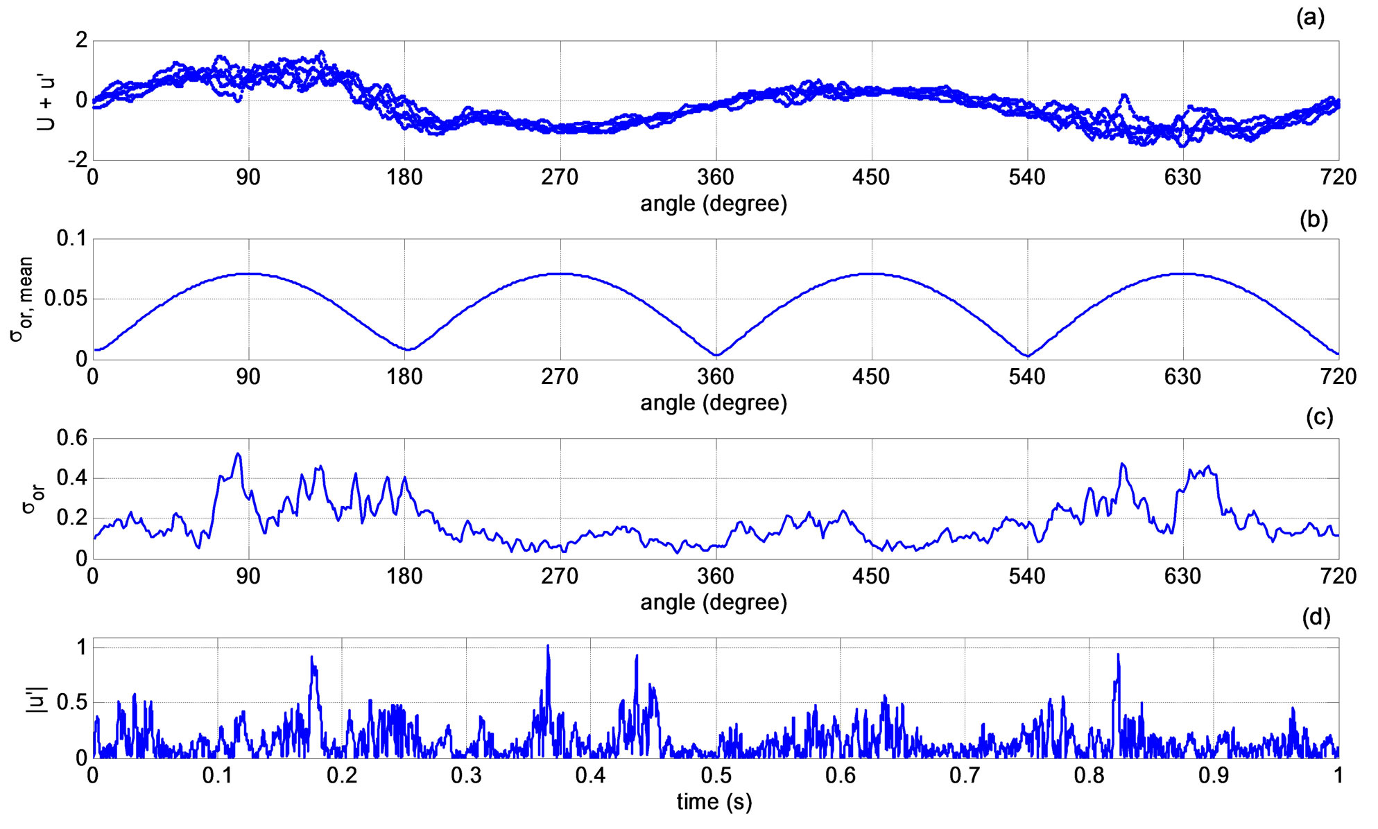
Figure 6. Simulated signal statistics: (a) signal velocity distribution with crank angle; (b) mean velocity standard deviation (Equation (9)) calculated using the original mean and the ensemble averaged mean velocity; (c) standard deviation variation with the crank angle; (d) absolute value of the fluctuating velocity in time.
 (12)
(12)
where  describes an ensemble averaged variation of the fluctuating velocity signal (Figure 6(c)), the
  defines a single standard deviation value for the fluctuating velocity signal (
 0.205 for the current signal). The
  shows the variations of the signal from the mean in the absolute sense (Figure 6(d)).
3. Analysis Methods-Description/Discussion
Different methods used in the analysis of the simulation signal were, ensemble averaging, high-pass filtering, Proper Orthogonal Decomposition (POD) also known as Principal Component Analysis (PCA) [41], Wavelet Decomposition (WD), WD and PCA together (WD/PCA). In this section these methods are described and some analysis results about their use are given.
Methods discussed in this section are the most commonly used methods in the analysis of cycle-to-cycle variation of engine data. Usually multiple techniques are employed within the same research. While the ensemble-averaging method is the most commonly used method [5,27,42-45], high-pass filtering method has been frequently employed [22,27,28,44-46]. Literature survey indicates that POD, WD and the WD/PCA methods have been less frequently employed [3,18,20-25].
Previous research on cyclic variability indicates that the time varying velocity in highly unsteady IC engine flows has usually been expressed as sum of mean and fluctuating components, . In general, the mean velocity component is considered as the component causing the cyclic variability in the signal; although cyclic variability in the fluctuating velocity has also been contemplated [28,29]. The methods used by different researchers differ in how the mean and the fluctuating velocities are determined.
In ensemble-averaging method it is assumed that the mean velocity does not vary from one cycle to the next and arithmetic averages of the velocities at specified crank angle intervals can be used to describe the mean velocity variation, .
.
In the high-pass (hp) filtering method [27], (named as “cycle resolved analysis” by Liou and Santavicca, [44] and Fraser and Bracco [45]; named as “cyclic averaging” by Sulivan et al. [22], time varying velocity signal is filtered at a pre-determined cut-off frequency to calculate the low-pass (lp) filtered signal and this signal is referred to as the mean velocity signal,
 . A variant of this technique uses a polynomial curve fitting to obtain the mean velocity component [47].
Another variant of high-pass filtering method, named as “filtered ensemble averaging” by Fansler [28] (named as “phase averaging”, Erdil et al. [3]), uses three terms to describe the velocity signal. In this method the difference between the low-pass filtered velocity and the ensemble-averaged mean velocity is defined as low frequency (LF) fluctuating velocity and the u’(t) is then considered as composed of a high frequency (HP) component, . In this variant the mean velocity is defined as,
 , and the fluctuating velocity as,
 . In essence high-pass filtering and the filtered ensemble averaging methods are equivalent to each other, and in each method different cut-off frequencies could be used at each cycle; although usually one frequency is used for the whole signal.
In the WD method the velocity signal is decomposed into “details”, where the sum of the details gives the original velocity signal. The fluctuation velocity information contained in the “detail” decreases with the increasing “detail” level. In this technique a high order “detail” is considered as the mean velocity signal.
In the POD method, velocity signal is re-expressed using new axes found as the eigenvectors of a covariance matrix formed using the velocity signal. The eigenvectors and the associated eigenvalues describe new coordinate axes on which the data lie the closest; the larger the eigenvalue the closer the data is to the eigenvector. In a reverse transformation to the original axes, neglecting the variations of signal along the axes with low eigenvalues allows defining the mean velocity component. In the WD/PCA method first the velocity signal is decomposed into details and then the POD is applied on these details. Similar to the WD method a high order detail is then considered as the mean velocity signal.
Additional unique methods, such as “turbulence filtering” by Erdil et al. [3], discuss possibility of separating the mean and the fluctuating velocities within the frequency domain using a filter function. In the current research, both the mean and the fluctuating velocities were considered to be time dependent and both were considered to have cyclic variations. In each method fluctuating velocity signals were next used to study turbulence statistics.
3.1. Ensemble Averaging
In the ensemble averaging method, time dependent velocity is defined as the sum of the ensemble-averaged mean velocity and the fluctuating velocity:
 (13)
(13)
where,  , is the crank angle;
  denotes average value;
 , are the prescribed crank angles at which the mean velocity values are calculated. Ensemble averaging assumes that the mean flow variation from one cycle to another is negligible and an average velocity value can be used to represent the mean value at a crank angle. The average velocity at a crank angle is calculated as the arithmetic mean of the velocity values within a prescribed crank angle interval:
 (14)
(14)
 ;
; ;
;  is the number of samples in the range
  for the whole duration of the signal. The
  (Equation (14)) is different than the
  (Equation (8)), since the ensemble averaged mean velocity is obtained using the composite signal rather than the mean velocity variation alone. Figure 7(a) shows both ensemble averaged meanvelocity variations calculated using the composite signal and using only the mean component of the composite signal (shown as smooth line).
A standard deviation is calculated using the differences between the ensemble-averaged mean velocity and the mean velocity of the original signal at the prescribed crank angles using the whole duration of the signal as:
 (15)
(15)
Figure 7(b) shows the  variation calculated using Equation (15). The variation shown is different than the variation shown in Figure 6(b) calculated using Equation (9) due to the differences in the mean velocity definitions used. Figure 7(b), as Figure 6(b), indicates to the fact that ensemble averaging results in large velocity fluctuations due to predicting the mean velocity variation incorrectly by ignoring cycle-to-cycle variations. The difference between the original signal mean and the ensemble mean (Equation (14)) results in a fluctuating signal.
The fluctuating velocity is next used to obtain standard deviation of the fluctuating velocity at prescribed crank angles:
 (16)
(16)
A standard deviation,  using the whole signal is calculated by:
 (17)
(17)
Figure 7(c) shows the difference between the standard

Figure 7. (a) ensemble averaged mean velocity variations,  and
and ; (b)
; (b)  given by Equation (15); (c) difference between
  and the
  nondimensionalized by
 .
.
deviations for the fluctuating velocities normalized by the standard deviation of the original signal.
In the application of the technique, simulated data with prescribed durations were used to calculate the mean velocity and the standard deviation variation with crank angle. Calculated variations for different signal durations differ from each other since the simulated signal contains cyclic variations that affect the calculated values. Calculation of the mean and the standard deviation variation by averaging the data values over the span of the signal rules out the use of the technique to obtain time-resolved variations.
3.2. High-Pass Filtering
In the high-pass filtering method the simulated signal is split into high and low frequency components at a cut-off frequency, fc, chosen by observation (fc = 30 Hz). The time dependent signal is low-pass filtered to obtain the mean velocity variation in time,  (Figure 8(a)). The difference between the original signal and the low-pass filtered signal is considered to be the fluctuating velocity signal.
 (18)
(18)
In the present work a single frequency value is used for the full length of the signal to separate the low and the high frequency contents. A Fast-Fourier-Transform is applied to the original signal to determine the power spectrum of the signal and to subsequently determine a cut-off frequency. The original time series signal was next filtered using a sixth order Chebyshev filter in the time domain to obtain the low frequency component. A relation exists between the mean velocity differences and the fluctuating velocity differences calculated using the original velocity signal and the velocity signals calculated by the method:
 (19)
(19)
Velocity differences are presented in Figure 8(b). High frequency signal was then used to calculate the fluctuating velocity standard deviation at different crank angles, and an overall average standard deviation:
 (20)
(20)
 (21)
(21)
Cut-off frequency fc = 30 Hz, results in  = 0.1957. Different cut-off frequency values result in different
  values; for fc = 10, 15, 20, and 25 Hz, the standard deviations are
  = 0.3441, 0.2426,

Figure 8. (a) Mean velocity variation obtained using high-pass filtering method and the simulated signal mean velocity variation (solid line in red); (b) Variations of , and
, and  with time; (c) difference between
  and the
  nondimensionalized by
 .
.
0.2223, and 0.2129, respectively. With the use of a 5 second long signal the values obtained for the fc = 10, 15, 20, 25 and 30 Hz, are  = 0.2604, 0.2119, 0.2102, 0.1954, 0.1788 respectively, indicating that the signal length does have an effect on the values calculated, but the effect is not significant at high frequency end.
Figure 8(a) shows the mean velocity calculated by the high-pass filtering technique and the mean velocity variation of the original signal in time. Figure 8(c) shows the difference between the standard deviations for the fluctuating velocities normalized by the standard deviation of the original signal.
3.3. Proper-Orthogonal Decomposition (POD)
The proper orthogonal decomposition (POD) was first introduced by Lumley [48] to identify coherent structures in turbulent flows. POD, also known as the Principal Component Analysis technique [41] allows one to represent data points each defined with N coordinates in a new N dimensional coordinate system such that the data points now lie closer to the new axes, allowing variations along preferred directions to be determined [49]. For example data maybe the realization of three fluctuating velocity components obtained in time, where the fluctuating velocities are the coordinates defining the data point obtained in time. In the representation of the data in the new coordinate system, the axes are sorted such that the data lie closer to the first axis than the other axes and the data lie closer to the second axis than to the third axis and so on. Representation with the new variables is sometimes referred to as sorting the data by their energy content. One of the advantages of the POD technique is that after the representation of the data in the new coordinate system, one can then approximate the data by reducing the number of coordinates used, say by neglecting the less energetic coordinates in representing the data. For more details and examples of POD technique on fluid mechanics measurements, the reader is referred to Tropea et al. [50].
In the numerical calculations of the POD technique multiple signals collected simultaneously are first stored in a data matrix,  , and the data matrix is then used to calculate a covariance matrix.
 (22)
(22)
where,  denotes the average of the data values in the ith row, thus
  is a different value for each row; superscript T denotes the transpose of the matrix; covariance matrix,
  is an M × M square matrix.
The next step is calculation of the eigenvalues and the eigenvectors of the covariance matrix. Eigenvalues,  , where k = 1 to M, and the eigenvector matrix
 , where i = 1 to M and k = 1 to M, of the covariance matrix, are calculated using Matlab. An eigenvector corresponding to an eigenvalue,
  is listed in the kth column of the eigenvector matrix
 . The eigenvectors of the covariance matrix correspond to the set of orthogonal axes (new coordinates) to represent the data. Once the eigenvectors are sorted in order corresponding to the eigenvalues of the covariance matrix, the projection of the original data along the eigenvector directions represents the data in these new orthogonal coordinates. During the process the sum of the square of the distances between the new axes (along the eigenvector directions corresponding to eigenvalues in descending order) and the data are minimized.
Projection of the original data along the direction of the unit eigenvectors can be obtained using:
 (23)
(23)
This process can be reverted to obtained the original signal , and can be recalculated using:
 (24)
(24)
The computations in Equation (24) also work if some of the eigenvectors corresponding to less energetic eigenvalues are omitted (set to zero) during the reversal process, leaving behind a signal close to the original signal that has been cleaned of outlier data points.
In the present work, first the complete velocity signal was converted into a data matrix,  , with each row of the matrix representing a full cycle of a four stroke engine spanning 720˚ of crank angle, with the first 720˚ signal (corresponding to the first cycle) in the first row, next 720˚ signal in the next row and so on. In describing
 , i = 1 to M, where, M represent the number of cycles used in the signal and j = 1 to N representing columns of the data corresponding to one full cycle of data spanning 720˚ of crank angle. Although this is strictly different than the conventional use of the POD technique, it allows working with a single dimensional data. Thus the data matrix is generated as if different cycle velocities were acquired simultaneously, resulting in velocities corresponding to same crank-angle to be listed in a single column. Presenting one dimensional data in an array allows using each cycle velocity value as a separate coordinate in the POD process.
In the present work the mean velocity signal was calculated using the largest eigenvalue containing 92.2% of the energetic contributions to the signal (Figure 9(a)) and the contributions from other eigenvalue/eigenvector couples were considered as turbulence contributions. The five eigenvalues obtained in the increasing order are 108.6, 150, 236.7, 280.9, and 2735.7. The contributions for the eigenvalues for a 10 second signal results in 50 eigenvalues, and the approximation improves with the simulated signal duration (discussed in Section 4.1).
In the POD method time dependent velocity is defined as the sum of the mean and the fluctuating velocity components:
 (25)
(25)
Statistical quantities are defined similar to other method statistical quantities:
 (26)
(26)
 (27)
(27)
 (28)
(28)
Figure 9(b) shows the difference between the mean velocities and the fluctuating velocities for the original signal and the ones calculated by the POD technique. Figure 9(c) shows the difference between the standard deviation calculated using the POD technique and standard deviation of the original fluctuating velocity normalized by the standard deviation of the original signal.
3.4. Wavelet Decomposition
Wavelet transformation determines the correlations between the original signal and the prescribed wavelet function at different frequency ranges of the original signal [51]. Following the description used by Farge [52] continuous wavelet transform is defined as the convolution of a wavelet , with the original signal to determine the wavelet coefficients,
 (29)
(29)
where
 (30)
(30)
“a” denotes the scale of the wavelet and related to the frequency of the signal, “b” is time value used in translating the wavelet;  is the daughter wavelets generated by translating and dilating (scaling) the mother wavelet. The wavelet coefficients thus calculated can be used to approximate the original signal at different scales. Reconstruction of the original signal is obtained using linear combination of the wavelet and the wavelet coefficient
 (31)
(31)

Figure 9. (a) Mean velocity variation obtained using the POD and the simulated signal mean velocity variation (solid line in red); (b) Variations of , and
, and  with time; (c) difference between
  and the
  nondimensionalized by
 .
.
where , is a constant and depends on the wavelet used. The coefficients with small scale values correspond to high frequency component of the signal and the ones with larger scale values correspond to low frequency values. During the reconstruction of the signal, length scales corresponding to the high frequency content can be omitted to obtain the low frequency (or mean) variation of the original signal. A history and a formal description of the wavelet transforms can be found in articles by Farge [53] and Tropea et al. [50].
While the mother wavelet can be presented in a functional form for a simple wavelet such as the Haar wavelet, in general an algebraic functional form does not exist. The mother wavelet , which can be a real or complex valued function, is chosen to satisfy multiple conditions, such as admissibility condition requiring that the energy contained within the wavelet to be a limited value, zero mean condition requiring the wavelet to have a zero mean value, and a requirement that its higher order moments vanish [53].
In the discretized wavelet transform the scale and the position “t” are described using powers of 2. Matlab [54] gives details about the discrete wavelet transform and the reader is referred to this document for further details. For a continuous signal , the discrete wavelet transform is given as:
 (32)
(32)
where  and the transformation gives the wavelet coefficients,
 . The original signal can be recovered without any loss using the inverse transform:
 (33)
(33)
For a fixed value of j, summation on the k gives the “detail” at the jth level:
 (34)
(34)
and thus,
 (35)
(35)
An approximation to the signal can be made using a limited number of details. For example  can be separated into two components, one using indices j ≤ J, corresponding to the scales,
  and one with j > J.
 (36)
(36)
If desired, the reconstructed signal could then be expressed only as “approximation”, Ai, at level J. A relation exists between different approximations as:
 (37)
(37)
Increasing values of J indicates that lesser details are used in generating the approximate signal, thus the approximation becomes closer to signal’s mean variation. The value of J should also not be chosen large such that the details in the mean variation are also sacrificed.
In the current work Daubechies 12, Symlet 8, and Coiflet 5 wavelets were tested and the results obtained did not vary with the use of different wavelets. Thus Daubechies 12 wavelet was chosen for further analysis of the data. Figure 10 shows the scaling and the wavelet functions for the Daubechies-12 wavelet.
In the wavelet decomposition time dependent velocity is thus defined as an approximation plus the details:
 (38)
(38)
where , and J =
8. Figure 11(a) presents the  and the original mean velocity variation in time.
Statistical quantities are calculated using:
 (39)
(39)
 (40)
(40)
 (41)
(41)
Figure 11(a) shows the original mean velocity and the mean velocity calculated by the WD technique. Figure 11(b) shows the mean and the fluctuating velocity differences, Figure 11(c) shows the difference between the standard deviation calculated using the WD technique and standard deviation of the original fluctuating velocity normalized by the standard deviation of the original signal.
3.5. Principal Component Analysis and Wavelet Decomposition
In this analysis method the advantages of the Principal Component Analysis and the Wavelet Decomposition methods are used simultaneously [55]. In the technique first wavelet decomposition is applied on the signal to calculate the “details” and one “approximation” to the signal. Next PCA analysis is employed on each of the detail signals and the approximation. PCA analysis results are used to determine which principal components to keep in the signal using the Kaiser rule. Kaiser rule keeps only the eigenvalues, which have values greater than the mean of all eigenvalues in re-construction of the signal. As a next step the details and the approximation reconstructed using the PCA are used in the reconstruction of the signal using the wavelet decomposition. In the detection of the mean velocity signal the wavelet decomposition allows the signal to be analyzed at different scales and the principal component analysis allows de-noising of the signal at every detail.
In the WD/PCA method time dependent velocity is defined as the sum of the mean and the fluctuating velocity components,
 (42)
(42)
Statistical quantities are defined using,
 (43)
(43)
 (44)
(44)
 (45)
(45)
 (a) (b)
Figure 10. (a) scaling and (b) the wavelet functions for Daubechies-12 wavelet.

Figure 11. (a) Mean velocity variation obtained using the WD and the simulated signal mean velocity variation (solid line in red); (b) Variations of , and
, and  with time; (c) difference between
  and the
  nondimensionalized by
 .
.
Figure 12(a) shows the original mean velocity and the mean velocity calculated by the WD technique. Figure 12(b), shows the mean and the fluctuating velocity differences, Figure 12(c) shows the difference between the standard deviation calculated using the WD/PCA technique and standard deviation of the original fluctuating velocity normalized by the standard deviation of the original signal.
4. Results and Further Discussion
A comparison between the Figures 8(a), 9(a), 11(a), and 12(a) show that all the mean velocity variations calculated by different methods follow the general variations observed in the simulated signal. Figures 8(b), 9(b), 11(b), and 12(b) show the differences of the mean and the fluctuating velocities between the original velocity components and the components calculated after each method, and give a sense of how well the methods perform in describing both the mean velocity and the fluctuating velocity vs. the crank angle. If a method could perfectly separate the mean and the fluctuating velocity values in time then the plots would be a straight line at zero. Figures indicate that the differences between the velocity signals are the smallest using the WD/PCA method, and that the POD method results contain high frequency content. POD performance improves with increased signal duration and the high frequency diminishes.
Figures 7(c), 8(c), 9(c), 11(c), and 12(c) show the normalized difference between the computed and the original signal standard deviations. Figures 8(c) and 11(c) indicate that the high-pass filtering and the WD techniques result in larger differences between the standard deviations than the other methods. The differences between the fluctuating and the mean velocities obtained using the original simulated velocity signal and the velocities computed after each method both contribute in the calculation of the fluctuating velocity standard deviation. This is due to the fact that the difference between the original velocity signal and the calculated mean velocity signal is considered as a contribution to the fluctuation velocity calculated by a method. For the 1 second analysis results shown in the figures, large non-dimensional differences are observed at locations where the original  values are small such as in the 250˚ - 280˚ and 450˚ - 500˚ ranges. Overall, the WD/PCA technique results follow the original standard values better than the other techniques.

Figure 12. (a) Mean velocity variation obtained using the WD/PCA and the simulated signal mean velocity variation (in red); (b) Variations of , and
, and  with time; (c) difference between
  and the
  nondimensionalized by
 .
.
4.1. Simulated and Calculated Signal Correlation —Effect of Signal Duration
In order to quantitatively determine the performance of each method in separating the mean and the fluctuating velocity variations, and the signal duration required to effectively separate the mean and the fluctuating velocity signal components correlation coefficients were calculated between the original simulation signal and the calculated signals. Correlation coefficients were calculated using:
 (46)
(46)
and
 (47)
(47)
A correlation coefficient of 1 indicates a perfect match between the two signals. Correlation coefficients calculated for signal durations of 0.6 s to 10.2 s with 0.6 s increments plotted in Figure 13 indicate that the WD/PCA method performs better than the other methods in calculating the mean and the fluctuating velocity signals. Both Figures 13(a) and (b) indicate that the performance of the methods get better with increased signal duration. Results do not show appreciable improvement after the first 3 seconds, and the changes after 8 seconds are minimal indicating that 3 seconds of data could be sufficient to extract the mean and the fluctuating velocity signals. Plots in Figures 13(a) and (b) show similar variations since poor mean velocity prediction by a method directly reflects on the fluctuating velocity prediction performance of the technique. Results also indicate that the WD and the high-pass filtering methods predict the mean and the fluctuating velocity variations poorly even with increased signal duration. Correlation coefficients as low as 0.8 obtained for the fluctuating signal indicate that the time variation of the fluctuating velocity calculated by these methods is a poor representation of the original fluctuating velocity signal. Figure 13(b) shows that the correlation coefficient values calculated even with the WD/PCA method is about 0.95 indicating to the need for further improved methods for accurate time variation prediction of the fluctuating velocity signal.
Figure 14 shows the ratio of the average standard deviations calculated by each method to the original signal average standard deviation for a given duration of signal. Normalized standard deviation (NSD) was calculated using:
 (48)
(48)
Figure 14 indicates that the standard deviation calculated by the WD/PCA method is approximately the same as the  once a 5 s signal duration is used. All the other methods except the ensemble-averaging method underestimate the
 ; ensemble averaging method


Figure 13. Correlation coefficient values obtained between the simulated mean and the simulated fluctuating velocity signals and the mean and fluctuating velocity components obtained by analysis methods. (a) mean velocity; (b) fluctuating velocity results.

Figure 14. Ratio of the average standard deviations calculated by each method to the original signal average standard deviation for a given duration of signal.
overestimates the  by a few percent. The NSD values calculated using the high-pass filtering and the WD methods show a performance decrease followed with a performance increase with the increased sample duration. POD values monotonically increase with the signal duration and reach a plateau at about 5 seconds. Results indicate that a signal with 5 s duration together with the WD/PCA method could be used to accurately estimate the
 ; although the
  achieved after 3 seconds is within a few percent of the
 .
.
4.2. Effect of Fluctuating Velocity σor,ave on Method Performance
The effect of the fluctuating velocity overall magnitude in the performance of the methods was investigated next by varying the signal  and calculating correlation coefficients for the mean and the fluctuating components using the Equations (46) and (47). Comparisons were made for 1 second and 5 second duration signals (Table 4). Results indicate that POD and the WD/PCA methods are superior to the high-pass filtering and the WD methods. While the WD/PCA works better than the POD method once the signal standard deviation is as same as the original
  and 2
and 2 , POD method works better once the signal standard deviation is 4
 and once a longer duration signal is used. For the signals with 1/2
 and 1/4
 the mean velocity signal is predicted well by all the methods. For these cases the POD and the WD/PCA methods predict the fluctuating velocity signal better than the other methods with better predictions by the POD technique once a longer period signal is used. Fluctuating velocity prediction capability decreases for all the methods with decreasing
  values.
4.3. Effects of Imposing Cyclic Variation on Fluctuating Velocity on Method Performance
Additional calculations were made to check the effect of imposing cyclic variations on the fluctuating component of the signal as described in Section 2.2 on the performance of the methods. For this purpose another fluctuating signal without the cyclic variations was generated. This signal uses only the filtered Gaussian signal without the cyclic variations. The amplitude of this new signal was adjusted to re-obtain the standard deviation of the experimental data. In this case the turbulence signal was defined as:
 (49)
(49)
The constant multiplier was used to match the standard deviations of this signal, the experimental data and the original fluctuating velocity signal. The analysis methods were then used to determine the performance of each method by calculating the correlation coefficients between the original mean and fluctuating signals and the signals obtained after the use of methods. The correlation coefficients for the mean signals obtained with the cyclic variation and without the cyclic variation vary less than 0.2%, while the correlation coefficients for the fluctuating signals vary less than 1% with less correlation coeffi-

Table 4. Correlation coefficients obtained between the simulated the calculated velocity by different analysis methods for 1 second (first row) and 5 seconds (second row) signal for different σor,ave values.
cient values without the cyclic variations imposed.
5. Conclusions
Performances of several methods were tested in separating the mean and the turbulent fluctuations of a simulated signal. Simulated signal was described using LDV data obtained in an IC engine and using a prescribed power spectrum. The results were presented using 1 second signal duration. Additional runs were made to see the effects of the signal duration and the fluctuating velocity standard deviation in the performance of the methods. Ensemble averaging technique is observed as a method that is not suitable for unsteady flow estimation since it can result in an artificial fluctuation velocity due to the cyclic variations that might be present in the mean velocity signal. High-pass filtering technique requires selection of a cut-off frequency for the signal; simulated signal characteristics could not be obtained after testing multiple cut-off frequencies. Presentation of the velocity or the turbulence in a coordinate system using the crank angle as the abscissa seems to be inappropriate in describing the unsteady flow since it hinders much of the details in the signals.
The correlation coefficients calculated using the original and the calculated mean and fluctuating velocities show that the WD/PCA and the POD methods perform better than the other methods. Correlation coefficients calculated by every method increase with increasing signal duration, predictions by the POD and the WD/PCA methods become closer to each other with better predictions by the WD/PCA technique.
The signal duration required to accurately separate the velocity components were investigated by varying the simulated signal duration. Correlation coefficient values calculated close to 1 using mean velocity signals and 5 s signal duration indicate that mean velocity calculated using POD and WD/PCA methods match the simulated mean velocity signals. For this signal duration, using the fluctuating velocity signals and the POD and the WD/ PCA methods result in correlation coefficients of about 0.95. Normalized standard deviations determined by different methods indicate that ~5 seconds of data is sufficient to estimate the standard deviation of the original signal using WD/PCA and the POD methods.
The effect of the fluctuating velocity magnitude was tested by varying the standard deviation value of the fluctuating velocity signal. For a 1 second data, results indicate that the WD/PCA and POD methods work better than the other techniques. The POD method seems to work better with a 5 s signal duration for signals with 1/2, 1/4 and 4 in predicting a signal variation closer to the simulated signal than the other methods.
Based on the correlation coefficient calculations made including signal duration and its magnitude the WD/PCA method seems to be the suitable method in separating the mean and the fluctuating velocity components of the signal studied. Conclusions reached here do not necessarily imply that the method is applicable to all unsteady flows but for a limited internal combustion engine flows.
6. Acknowledgements
P. A. Schinetsky was sponsored in Summer-2008 by the National Science Foundation Research Experience for Undergraduates University of Alabama site under NSF grant EEC 07554117.
REFERENCES
- L. J. Lumley, “Engines, an Introduction,” Cambridge University Press, Cambridge, 1999. doi:10.1017/CBO9781139175135
- E. P. Hassel and S. Linow, “Laser Diagnostics for Studies of Turbulent Combustion,” Measurement Science and Technology, Vol. 11, No. 2, 2000, pp. R37-R57. doi:10.1088/0957-0233/11/2/201
- A. Erdil, A. Kodal and K. Aydin, “Decomposition of Turbulent Velocity Fields in an SI Engine,” Flow, Turbulence and Combustion, Vol. 68, No. 2, 2002, pp. 91-110. doi:10.1023/A:1020467008591
- W. C. Choi and Y. G. Guezennec, “Experimental Investigation to Study Convective Mixing, Spatial Uniformity, and Cycle-to-Cycle Variation during the Intake Stroke in an IC Engine,” Journal of Engineering for Gas Turbines and Power, Vol. 122, No. 3, 2000, pp. 493-501. doi:10.1115/1.1286626
- A. R. Denlinger, Y. G. Guezennec and W. C. Choi, “Dynamic Evolution of the 3-D Flow Field during the Latter Part of the Intake Stroke in an IC Engine,” Analysis of Combustion and Flow Diagnostics (SP-1348), SAE paper, 1998.
- M. P. Patrie and J. K. Martin, “PIV Measurements of in-Cylinder Flow Structures and Correlation with Engine Performance,” Fall Technical Conference, 1997.
- H. J. NeuBer, L. Spiegel and J. Ganser, “Particle Tracking Velocimetry-A Powerful Tool to Shape the in-Cylinder Flow of Modern Multi Valve Engine Concepts,” SAE Paper, 1995.
- K. H. Lee, C. S. Lee, H. J. Park and D. S. Kim, “Effects of Tumble and Swirl Flows on the Turbulence Scale Near the TDC in 4 Valve SI Engine,” ICE Spring Technical Conference, 2001.
- D. P. Towers and C. E. Towers, “Cyclic Variability Measurements of in-Cylinder Engine Flows Using HighSpeed Particle Image Velocimetry,” Measurement Science and Technology, Vol. 15, No. 9, 2004, pp. 1917- 1925. doi:10.1088/0957-0233/15/9/032
- R. B. Rask, “Laser Doppler Anemometer Measurements in an Internal Combustion Engine,” SAE Paper, 1979.
- S. Bopp, F. Durst and C. Tropea, “In-Cylinder Velocity Measurements with a Mobile Fiber Optic LDV System,” SAE Paper, 1990.
- F. Durst, A. Naqwi and C. Tropea, “Development and Applications of LDA-systems in I.C. Engine Research,” International Symposium, Vol. 90, 1990, pp. 21-30.
- H. Vigor, J. Pecheux and J. L. Peube, “Velocity Measurements Inside the Cylinder of an Internal Combustion Model Engine during the Intake Process,” Laser Anemometry, Vol. 1, 1991.
- M. R. Himes and P. V. Farell, “Laser Doppler Velocimeter Measurements within a Motored Direct Injection Spark Ignited Engine,” University of Wisconsin-Madison, Madison, 1998.
- K. Y. Kang and J. H. Baek, “Turbulence Characteristics of Tumble Flow in a Four-Valve Engine,” Experimental Thermal and Fluid Science, Vol. 18, 1998, pp. 231,243.
- V. S. S. Chan and J. T. Turner, “Velocity Measurement Inside a Motored Internal Combustion Engine Using Three-Component Laser Doppler Anemometry,” Optics & Laser Technology, Vol. 32, 2000, pp. 557-566.
- B. Kim, et al., “In-Cylinder Turbulent Measurements with a Spark Plug-In Fiber LDV,” 11th Symposia on Applications of Laser Techniques to Fluid Mechanics, Lisbon, 8-11 July 2002.
- D. Park, P. Sullivan and J. Wallace, “Different Velocity Data Analysis for Flows Near a Spark Plug in the Combustion Chamber of a Spark Ignition Engine,” SAE Paper, 2004.
- C. Arcoumanis and J. H. Whitelaw, “Fluid Mechanics of Internal Combustion Engines: A Review,” International Symposium on Flows in Internal Combustion Engines-III, Vol. 201, No. 1, 1985, pp. 57-74.
- S. Roudnitzky, P. Druault, and P. Guibert, “Proper Orthogonal Decomposition of in-Cylinder Engine Flow into Mean Component, Coherent Structures and Random Gaussian Fluctuations,” Journal of Turbulence, Vol. 7, No. 70, 2006, p. 70.
- M. Fogleman, J. Lumley, D. Rempfer and D. Haworth, “Application of the Proper Orthogonal Decomposition to Datasets of Internal Combustion Engine Flows,” Journal of Turbulence, Vol. 5, No. 23, 2004, pp. 1-18.
- P. Sullivan, R. Ancimer, J. Wallace, “Turbulence Averaging within Spark Ignition Engines,” Experiments in Fluids, Vol. 27, No. 1, 1999, pp. 92-101. doi:10.1007/s003480050333
- R. Ancimer, P. Sullivan and J. Wallace, “Decomposition of Measured Velocity Fields with Spark Ignition Engines Using Discrete Wavelet Transforms,” Experiments in Fluids, Vol. 30, No. 2, 2001, pp. 237-238. doi:10.1007/s003480000152
- F. Söderberg, B. Johansson, and B. Lindoff, “Wavelet Analysis of in-Cylinder LDV Measurements and Correlation Against Heat-Release,” SAE Paper, 1998.
- A. Sen, G. Litak, R. Taccani and R. Radu, “Wavelet Analysis of Cycle-to-Cycle Pressure Variations in an Internal Combustion Engine,” Chaos, Solitons and Fractals, Vol. 38, No. 3, 2008, pp. 886-893. doi:10.1016/j.chaos.2007.01.041
- Z. Zhang, E. Tomita, S. Yoshiyama, Y. Hamamoto and H. Kawabata, “Wavelet Transform Analysis of Unsteady Turbulence and Turbulent Burning Velocity in a Constant-Volume Vessel,” JSME International Journal, Series B, Vol. 44, No. 4, 2001, pp. 608-615. doi:10.1299/jsmeb.44.608
- C. Arcoumanis, A. C. Enotiadis and J. H. Whitelaw, “Frequency Analysis of Tumble and Swirl in Motored Engines,” Journal of Automobile Engineering, Vol. 205, 1991, pp. 177-184. doi:10.1243/PIME_PROC_1991_205_168_02
- T. D. Fansler, “Turbulence Production and Relaxation in Bowl-in-Piston Engines,” SAE Paper, 1993.
- A. C. Enotiadis, C. Vafidis and J. H. Whitelaw, “Interpretation of Cyclic Flow Variations in Motored Internal Combustion Engines,” Experiments in Fluids, Vol. 10, No. 2-3, 1990, pp. 77-86.
- E. Esirgemez and M. S. Ölçmen, “Spark-Plug LDV Probe for in-Cylinder Flow Analysis of Production IC Engines,” Measurement Science and Technology, Vol. 16, No. 10, 2005, pp. 2038-2047. doi:10.1088/0957-0233/16/10/020
- N. Kevlehan, J. C. R. Hunt and J. C. Vassilicos, “A Comparison of Different Analytical Techniques for Identifying Structures in Turbulence,” Applied Scientific Research, Vol. 53, No. 3-4, 1994, pp. 339-355. doi:10.1007/BF00849109
- H. E. Albrecht, M. Borys, N. Damaschke and C. Tropea, “Laser Doppler and Phase Doppler Measurement Techniques,” Springer-Verlag, 2003.
- L. H. Benedict, H. Nobach and C. Tropea, “Estimation of Turbulent Velocity Spectra from Laser Doppler Data,” Measurement Science and Technology, Vol. 11, No. 8, 2000, pp. 1089-1104. doi:10.1088/0957-0233/11/8/301
- E. Konstantinidis, A. Ducci, S. Balabani and M. Yianneskis, “An Empirical Method for Efficient Spectrum Estimation from LDA Data,” 13th International Symposiaon Applications of Laser Techniques to Fluid Mechanics Lisbon, Portugal, 26-29 June 2006.
- I. Çelik, I. Yavuz, A. Smirnov, J. Smith, E. Amin and A. Gel, “Prediction of in-Cylinder Turbulence for IC Enginess,” Combustion Science and Technology, Vol. 153, No. 1, 2000, pp. 339-368. doi:10.1080/00102200008947269
- “Matlab,” version 7.7.0.471, The MathWorks Inc., Natick, 2008.
- P. M. T. Broersen and S. de Waele, “Generating Data with Prescribed Power Spectral Density,” IEEE Transactions on Instrumentation and Measurement, Vol. 52, No. 4, 2003, pp. 1061doi:10.1109/TIM.2003.814824
- S. F. Al-Sharif, M. A. Cotton and T. J. Craft, “Reynolds Stress Transport Models in Unsteady and Non-Equilibrium Turbulent Flows,” International Journal of Heat and Fluid Flow, Vol. 31, No. 3, 2000, pp. 401-408. doi:10.1016/j.ijheatfluidflow.2010.02.024
- S. He, C. Ariyaratne and A. E. Vardy, “A Computational Study of Wall Friction and Turbulence Dynamics in Accelerating Pipe Flows,” Computers & Fluids, Vol. 37, No. 6, 2008, pp. 674-689. doi:10.1016/j.compfluid.2007.09.001
- A. J. Revell, S. Benhamadouche, T. Craft and D. Laurence, “A Stress-Strain Lag Eddy Viscosity Model for Unsteady Mean Flow,” International Journal of Heat and Fluid Flow, Vol. 27, No. 5, 2006, pp. 821-830. doi:10.1016/j.ijheatfluidflow.2006.03.027
- Y. C. Liang, H. P. Lee, S. P. Lim, W. Z. Lin, K. H. Lee and C. G. Wu, “Proper Orthogonal Decomposition and Its Applications—Part I: Theory,” Journal of Sound and Vibration, Vol. 252, No. 3, 2002, pp. 527-544.
- E. Zervas, “Correlations between Cycle-to-Cycle Variations and Combustion Parameters of a Spark Ignition Engine,” Applied Thermal Engineering, Vol. 24, No. 14-15, 2004, pp. 2073-2081. doi:10.1016/j.applthermaleng.2004.02.008
- W. C. Choi and Y. G. Guezennec, “Study of the Flow Field Development During the Intake Stroke in an IC Engine Using 2-D PIV and 3-D PTV,” International Congress and Exposition Detroit, Michigan, 1-4 March 1999.
- T.-M. Liou and D. A. Santavicca, “Cycle Resolved LDV Measurements in a Motored IC Engine,” Journal of Fluids Engineering, Transactions of ASME, Vol. 107, 1985, pp. 232-240.
- R. A. Fraser and F.V. Bracco, “Cycle-Esolved LDV Integral Length Scale Meaurements Investigating Clearance Height Scaling, Isotropy, and Homogeneity in an I.C. Engine,” International Congress and Exposition, Detroit, 27 February-3 March 1989.
- C. W. Hong and D. G. Chen, “Direct Measurements of in-Cylinder Integral Length Scales of a Transparent Engine,” Experiments in Fluids, Vol. 23, No. 2, 1997, pp. 113-120. doi:10.1007/s003480050092
- R. B. Rask, “Comparison of Window, Smoothed-Ensemble, and Cycle-to-Cycle Data Reduction Techniques for Laser Doppler Anemometer Measurements of in-Cylinder Velocity,” In: T. Morel, R. P. Lohmann and J. M. Rackley, eds., Fluid Mechanics of Combustion Systems, ASME, New York, 1981.
- J. L. Lumley, “The Structure of Inhomogeneous Turbulence,” In: A. M. Yaglom and V. I. Tatarski, eds., Atmospheric Turbulence and Wave Propagation, Nauka, Moscow, 1967, pp. 166-178.
- A. Chatterjee, “An Introduction to the Proper Orthogonal Decomposition,” Current Science, Vol. 78, No. 7, 2000, pp. 808-817. C. Tropea, A. L. Yarin and J. F. Foss, “Springer Handbook of Experimental Fluid Mechanics,” 2007.
- C. Torrence, and G. P. Compo, “A Practical Guide to Wavelet Analysis,” Bulletin of the American Meteorological Society, Vol. 79, No. 1, 1998, pp. 61-78. doi:10.1175/1520-0477(1998)079<0061:APGTWA>2.0.CO;2
- M. Farge, K. Scheineder and P. Abry, “Analyzing and Compressing Turbulent Fields with Wavelets,” Institut Pierre Simon Laplace Publication, 2002.
- M. Farge, “Wavelet Transforms and Their Applications to Turbulence,” Annual Review of Fluid Mechanics, Vol. 24, 1992, pp. 395-457. doi:10.1146/annurev.fl.24.010192.002143
- M. Misiti, Y. Misiti, G. Oppenheim and J.-M. Poggi, “Wavelet Toolbox™ 4, User’s Guide,” 2008.
- M. Aminghafari, N. Cheze and J.-M. Poggi, “Multivariate Denoising Using Wavelets and Principal Component Analysis,” Computational Statistics & Data Analysis, Vol. 50, No. 9, 2006, pp. 2381-2398. doi:10.1016/j.csda.2004.12.010