International Journal of Geosciences
Vol. 3 No. 3 (2012) , Article ID: 21194 , 16 pages DOI:10.4236/ijg.2012.33056
Geo-Electrical Investigation of Mullusi Aquifer, Rutba, Iraq
1Center of Desert Studies, University of Anbar, Ramadi, Iraq
2Department of Applied Geology, University of Anbar, Ramadi, Iraq
Email: *ealheety@Yahoo.com
Received January 10, 2012; revised April 1, 2012; accepted May 12, 2012
Keywords: Geo-Electrical; Layer; Hydraulic Conductivity; Mullusi Aquifer; Iraq
ABSTRACT
The geophysical study was performed east of Rutba town due to vertical electrical sounding in a net of forty points between Dhalaa and Dhabaa valleys. Geophysical electrical model applicated using Winsev6 program to determine the geo-electrical layers. Three geo-electrical layers were derived from geophysical survey. These layers are composed of four sediment types, such as clays, marls, marly carbonates, carbonates (dolomitic limestone), characterized by resistivity less than 20 ohm-m, 20 - 100 ohm-m, 100 - 350 ohm-m and more than 350 ohm-m, respectively. The thickness of the geo-electrical horizons are increased in Dhabaa Fault zone which characterized by multi karst shapes reflected as karst topography on the surface, which represents subsurface structural boundary for Mullusi aquifer, where this aquifer considered as main water supply for Rutba people in drinking water throughout 17 water wells located in Dhabaa site. Two empirical relation between Formation Factors (F) and Hydraulic Conductivity (K) obtained using linear and Polynomial regression techniques. The first equation of linear fit (F = 11.82 + 116.45 K; with a Correlation Coefficient of 0.94) represents the contribution between formation factor and hydraulic conductivity of a 2nd layer in Mullusi aquifer. The second equation of 3rd degree Polynomial Fit (F = 20.32 − 203.33 K + 1554.99 K2 − 3127.30 K3; with a Correlation Coefficient of 0.75) represents the contribution between formation factor and hydraulic conductivity of a 3rd layer in Mullusi aquifer.
1. Introduction
The initial application of electrical resistivity methods in geophysical prospecting started with the work of Wenner [1] and Schlumberger [2], both of whom proposed fourpoint electrode configuration for field measurements. A third general class of electrode arrays is the dipole-dipole array described by Alpin [3], for deep investigations .The electrical resistivity method is utilized in diverse ways for groundwater ([4-12]).
The purpose of this paper is to use the electrical resistivity data as vertical electrical sounding (VES) to study Mullusi aquifer conditions, such as depth, boundaries, water bearing horizons. Geo-physical survey aims to support the geological and hydrogeological data in determining the aquifer and their vertical and lateral extensions which are influenced by geological, structural and/ or geo-morphological settings. This is done by comparing the values of the electrical resistance of rocks, which represent their effectiveness to electric current passage and its relationship to the type of metal-forming layers and the amount of moisture in the pores as well as salt content, also determine the contribution of hydraulic conductivity (permeability) with formation factor includeing resistivity of groundwater and resistivity of saturated rocks (Mullusi aquifer).
2. Materials and Methods
The study area is located to the east of Rutba City, west of Iraq, between latitudes (32˚59'50" - 33˚03'48") and longitudes (40˚34'42" - 40˚24'44''), Figure 1, covers an area of about (112) km2, that extends between Al Dhalaa and Al Dhabaa valleys, with an elevation ranging between (575 - 616) meters above sea level , including the area where the system of water wells for Dhabaa water project consisting of 17 production wells, which are used for supply to the population of Rutba City, Figure 2.
Depending on the classification program of the United Nations Environment UNEP-1991 the region is climatically classified within the dry arid zone for the duration of the second half of the twentieth century [13].
2.1. Geology
Phisographically, the study area lies in the western part

Figure 1. Location map of geophysical survey.

Figure 2. 3 Model and topographic map of the study area.
of the upper valleys province to the east of Rutba city, and possibly classified as part of the transitional zone between the upper valleys and Al-Hammad provinces. Region is characterized by undulating terrain rises gradually from the east to the west. Decline in the Earth’s surface ranges between (0.07 - 13) m/km at a rate of decline of 2.05 m/km towards the north-east. From a geological perspective, the study area is characterized by its proximity to the Quaternary deposits , Rutba Sandstone Formation (Cenomanian-Upper Cretaceous), Maudud-Naher Umer Formations (Lower Cretaceous-Albian), Ubaid clayey dolomitic limestone (lower Jurassic), in addition to Mullusi dolomitic Limestone (Upper Triassic) [14]. The geological section of the study area can be seen in the sections of wells (W-1 and W-9), Figure 3. Structurally, the region is located at the southern limb of Horan anticline, whose fold axis extends along SW-NE direction.
The region is intersected by Dhabaa Fault that belongs to the system of Horan strike slip faults and extends with Dhabaa Valley of SW-NE direction, which is confirmed by Al-Mubarakstudy [15], while Al-Bassam et al. [16] classified Dhabaa Fault as normal fault with horizontal slip.
2.2. Electrical Resistivity Method
The electrical resistivity method depends on AC passage of low-frequency underground by a pair of metal electrodes installed on the Earth’s surface and measure the voltage between two electrodes are installed between them and all these poles are located on a straight line. Current flows emitted from pole and bend toward the other pole and be in vertical position on equipotential lines, which is distributed on a semi-spherical and its center position at the current poles [17]. Values of the measured voltage depend on the deployment location of the center poles and the distance between them and the direction of the path of the survey, in addition to the values of electrical conductivity of minerals and rocks layered solutions in pores [18]. Rock resistance values ranging from one to a few tens (ohm-m) in the mud and marl, and (10 - 1000) ohm-m in sand and sandstones, and more than 100 ohm-m in the limestone. The process of vertical electric sounding takes sequential measurements of the resistance by increasing the virtual distance between the poles of the current deployment, while the center of array and the trend remains constant [19]. This involves the principle of increased access current, by increasing of a deployment distance. The ratio between the depth of current penetration

Figure 3. Lithologic logs of W-1 and W-9.
and the distance between the electrodes is called penetration factor. The depth of current penetration is of about (1/4 to 1/3) the distance between the poles of power [20].
2.3. Vertical Electrical Sounding
Vertical electrical sounding provides information concerning the vertical succession of different conducting zones and their individual thicknesses and resistivities. By installing two electrodes into the ground and inducing an electric current through the ground, a potential field is created. Two additional electrodes are used to measure the potential at some location. Increasingly deeper measurements are achieved by using a larger separation between the current electrodes. Moving the current electrodes and having the potential electrodes fixed is named the Schulumberger array. In the electrical sounding with the Schulumberger array, the mid point of the electrodes array remains fixed but the spacing between the electrodes is generally increased to obtain more information about the deeper sections of the subsurface. For Schulumberger array, apparent resistivity is given by [21].
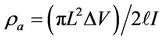
where, L = Half current electrode separation.
ℓ = Half potential electrode separation.
∆V = potential difference.
I = electrical current.
2.4. Data Acquisition
The sounding locations are shown in Figure 4. Forty Vertical electrical sounding (VES) were acquired using Schulumberger array with a maximum current electrode separation (2L or AB) of 350 meters. The instrument used was the SYSCAL R2 UNIT, IRIS Company, a digital averaging instrument for direct current resistivity work. Actual data acquisition begins with the selection of sounding point. Once the sounding location was determined, the instrument was deployed to the position. The geographic location and elevation of the chosen sounding point was measured by GARMIN SUMMIT-e TREX GPS apparatus. The vertical electrical sounding (VES) field data were processed using Winsev6, a computer iteration resistivity software and layers, which depends on the following geophysical references [22-26]. Detailed quantitative interpretation was done with the Winsev6 software.
3. Results and Discussion
The results of the VES interpreted through Winsev6 software are given in Table 1. A geo-electric layer is described by two fundamental parameters including its resistivity and thickness. The geo-electric sections for seventeen vertical electrical sounding (VES) indicate that there were two geo-electric layers as in VES-1, Figure 5. At the other vertical electrical sounding points, the geoelectric sections indicate that there were three geo-electric layers as shown in VES-5 for example, Figure 6.
3.1. Geo-Electrical Layers
Spatial distribution maps of resistivity , thickness and lithology of the three geo-electrical layers are outputted from the results of geophysical models, using a computer software (Surfer8 program), in addition to the three-dimensional models which explained the lower surface of each layer in the study area.
3.1.1. First Geo-Electrical Layer
In this layer, the values of apparent resistivity ranged between (9.5 - 1318) Ω-m, with an average of 193.5 Ω-m. The spatial distribution map of resistivity in this layer, Figure 7, showed heterogeneity in values of resistivity and increasing towards the south and south-east. The heterogeneity reflects the distribution of subsurface rock

Figure 4. VES points within study area.


Table 1. Resistivity and thickness of geo-electrical layers within Dhabaa region.
Formations, different soils resulting from erosion in the valleys and karsts. The resistivities of Ubaid Formation including marls, marly limestones and silty sandy clastic sediments of Naher Umer Formation are low and ranged between (10 - 170) Ω-m in the northern and north west parts, while the resistivities of dolomites and dolomitic limestone in Maudod Formation and sandstones of Rutba Formation are high and ranged between (170 - 1318) Ω-m, in the eastern part of region as shown in Figure 8. Thickness of the First geo-electrical layer ranged beween

Figure 5. Geo-electrical model and profile, VES-1.

Figure 6. Geo-electrical model and profile, VES-5.

Figure 7. Spatial distribution map of resistivity in 1st geo-electrical horizon within Dhabaa area.

Figure 8. Spatial distribution map of lithology in 1st geo-electrical horizon within Dhabaa area.
(22 - 119) meters, with an average of 48.5 meters. The iso-thickness map of this layer Figure 9, showed that there is a variation in the thickness of the layer increased in Dhabaa basin and the outcrop of Naher Umer Formation. Increasing of the thickness along Dhabaa valley basin, reflects elongated subsidence with maximum in (VES-7), and may be reflect Dhabaa fault zone intersecting the study area in the direction of north-south. Three dimensional model of the first geo-electrical layer Figure 10, showed that there is variation in the levels of the lower contact, oscillating between (468 - 586) m·asl, with slope ranging between 1 m/10 km - 95 m/1 km in Dhabaa downstream. It is symmetry to some extent with topography of land’s surface and this confirms the structural control on the terrain of the study area.
3.1.2. Second Geo-Electrical Layer
The apparent resistivity of the second layer ranged between

Figure 9. Iso thickness map of 1st geo-electrical horizon within Dhabaa area.

Figure 10. Spatial distribution map of 1st geo-electrical horizon (lower contact) within Dhabaa area.
(16 - 786) Ω-m, with an average of 168.5 Ω-m. The spatial distribution map of resistivity in this layer Figure 11, showed heterogeneity in values of resistivity and decreased towards Dhabaa valley to below 100 Ω-m, because of possibility of increasing the proportion of crushing in the rocks formation of Mullusi aquifer, due to the cavitations and subsidence processes resulting from weathering of carbonate rocks or from the fractures accompanied with Dhabaa Fault or both. The heterogeneity of resistivity reflects the difference in resistance of Mullusi rocks formation in proportion to the difference of marl from one region to another Figure 12, in addition to the difference in rocks porosity and the water content, where the results of pumping test indicated varied permeability values from one location to another.
The thickness of second layer ranged from 13 m to

Figure 11. Spatial distribution map of 2nd geo-electrical horizon within Dhabaa area.

Figure 12. Spatial distribution map of lithology in 2nd geo-electrical layer within Dhabaa area.
295 m with an average of 106.5 meters. The iso-thickness map of second geo-electrical layer Figure 13, showed variation in thickness values increased in Dhabaa hydrologic basin and the southwestern part of the study area, it may reach thickness of higher than 160 meters. Increasing of thickness along Dhabaa valley reflects subsidence with maximum value at the point (VES-28). The increased thickness may also reflect Dhabaa Fault zone in a direction of north east-south west and can be seen in Figure 14, which represents three-dimensional model of the lower surface level of the second layer. The lower surface of the 2nd layer varies and oscillates between levels of (260 - 540) meters above sea level with slope ranges between 7 m/10 km to higher slope of 207 m/1 km within Dhabaa basin. The lower surface of second layer is positively conformable with the lower surface of first layer, but the value of slope higher, which indicates a high probability of exposure to action weathering less

Figure 13. Iso thickness map of 2nd geoe-lectrical horizon within Dhabaa area.

Figure 14. 3D model of 2nd geoe-lectrical horizon (lower contact) within Dhabaa area.
than the first layer. The lower surface of second layer is negatively conformable with the lower surface of first layer in the other regions, and this leads to the promotion and confirmation of structural control on the terrain of study area.
3.1.3. Third Geo-Electrical Layer
The apparent resistivity of the third layer ranged between (1 - 829) Ω-m, with an average of 176.5 Ω-m. The spatial distribution map of resistivity in this layer. Figure 15 shows some homogeneity (less than average) in more than 80% of the study area. The resistivity decreases towards Dhabaa valley, where resistivity values down to less than 50 Ω-m, due to high percentage of clay minerals in Marlstone and/or water content in fracture Dolostones of Mullusi aquifer. The resistivity of the third layer in the western part of study area increases to 829 Ω-m, which reflects the characteristics of limestone and dolomitic limestone (free of clays) containing fresh water of Mullusi aquifer Figure 16. The thickness of the third geo-electrical layer ranged between (1 - 186) meters, with an average of 106 meters. The thickness map of this layer, Figure 17, showed increasing of thickness from 50 m to 170 m in the vicinity of the eastern and western regions of Dhabaa hydrologic basin, while thickness reaches less than 30 meter within the section of Dhabaa valley. In some areas the third geo-electrical layer disappears (thickness shall be zero). Three-dimensional model of the lower surface of the third layer, which represents the maximum value of electrical sounding obtained through geo-physical surveys is shown in Figure 18, the lower surface of the layer varies and oscillates from the level of 220 to 430 m·asl. with a gradient of 7 cm/1 km in most of the study area, while the maximum gradient is

Figure 15. Spatial distribution map of resistivity in 3rd geo-electrical horizon within Dhabaa area.

Figure 16. Distribution map of lithology of 3rd geo-electrical layer within Dhabaa area.

Figure 17. Iso thickness map of 3rd geo-electrical horizon within Dhabaa area.

Figure 18. 3D model and spatial distribution map of the lower surface of 3rd geo-electrical horizon.
equal to 133 meters/1 km at the survey point No. (VES- 28) in area classified as karstified topography with blind valleys.
Finally, the sections can be identified by geo-electrical layers of the study area, which obtained from the interpretation of resistivity model values which are compared to international standard resistance of the rocks and sediments as shown in Figure 19. The values of resistivity in Clay layers are of less than 20 ohm-m, while the values of the resistivity in Marl layers are of (20 - 100) ohm-m. The resistivity in calcareous Clay layers and marly Limestone are between (100 - 350) ohm-meters, while the resistivity of dolostone and limestone is more than 350 ohm-m. After obtaining the results of the values of resistivity and thickness of geo-electrical layers and compared with geological and hydrogeological information for the purpose of studying the aquifers and other water-bearing rock properties and the extent of variability (vertically and horizontally). It was found that the results of the models of interpretation was consistent with the properties of rocks and water content. The water table in the study area is not determined, and this may be attributed to the ambiguity of interpretation of the field geo-electrical curves. This ambiguity is interpreted in terms of equivalence and/or principle of suppression [19, 27]. The principle of suppression reflects presence of a layer that has a little thickness with intermediate resistivity relative to the up upper and lower layers. This layer does not show its effect on the field curve except in the case of increasing thickness. The principle of suppression reflects also presence of Marl or Clay layers above any aquifer. The behavior of electrical current in the marl and clay layer is similar to it in the aquifers, and this is what is happening mostly in the study area, where there is marl and clay in most of the stratigraphic sequence, that caused undetermining of the water table.
3.2. Contribution to the Knowledge of Aquifer’s Permeabilities
Geophysicists have realized that the integration of aquifer parameters calculated from the existed boreholes locations and resistivity parameters extracted from VES resistivity measurements can be highly effective, since a correlation between hydraulic and electrical aquifer properties can be possible, as both properties are related to the pore space structure and heterogeneity ([28-34]). The fundamental principle of the application of the geo-electrical methods in hydrogeology is the utilization of the dependence of rocks resistivity on the lithology and the mineralization of the water filling the pores. According to Equation (1) the resistivity of the saturated rock (ρws) is directly proportional to the resistivity of the water (ρw) filling the pores.
 (1)
(1)
where F is known as the formation factor. Thus, knowing the resistivity of groundwater, we can calculate F. Ground water resistivities and resistivity of the saturated rocks in Dhabaa Site were determined from 15 in situ measurements at wells distributed in the investigation
4. Conclusions
Based on the interpretation of geo-electrical data, the

Figure 19. Fence diagram showing the geo-electrical layers within study area.
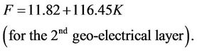
following conclusions are deduced: area, Tables 2 and 3. Measurements of the hydraulic conductivity (permeability) K were also made from pumping test analysis at each calibration borehole. Figures 20 and 21 show the plot of ( ) versus K for the 2nd and 3rd Geo electrical layers. Equations (2) and (3) is the empirical relation between F and K obtained by using linear and Polynomial regression techniques.
 (2)
(2)
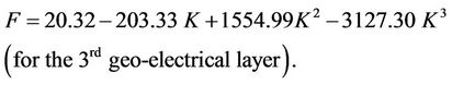
 (3)
(3)
Since drilling of wells to determine hydraulic parameters is often expensive, determining the aquifer parameters from VES is a cost-effective alternative. Based on our results, the contribution of VES coupled with the available pumping test data proved to be significant to the quantitative estimation of aquifer parameters.
1) Seventeen VES tests revealed two subsurface geoelectrical layers and twenty VES tests revealed three geoelectrical layers.
2) The apparent resistivity and thicknesses of geoelectrical layers were identified. The apparent resistivity of the first, second and third layers ranged between (9.5 - 1318) ohm-m, (16 - 786) ohm-m and between (1 - 829) ohm-m, respectively. While the thickness ranged between (22 - 119) meters, (13 - 259) meters and between

Table 2. Geo-electrical and hydraulic data of 2nd Layer.

Table 3. Geo-electrical and hydraulic data of 3rd Layer.

Figure 20. Formation factor versus permeability plot (2nd layer).

Figure 21. Formation factor versus permeability plot (3rd layer).
(1 - 186) meters for the first, second and third layer, respectively.
3) The subsurface lithology of the study area are identified based on VES tests, which consists of Clays, Marl, Marly Limestone, Dolostones and Dolomitic Limestones.
4) The iso thickness spatial distribution map indicated the horizontal and vertical heterogeneity of layers thickness, which increases within the zone of Dhabaa valley in karst topography of blind tributaries in the trend of Dhabaa fault of the northeast-southwest direction.
5) The following two equations represent the empirical relationship between Formation factor ( ) and hydraulic conductivity (permeability K) for the 2nd and the 3rd geo-electrical layers of Mullusi aquifer.
REFERENCES
- F. Wenner, “A Method of Measuring of Earth Resistivity,” Bulletin of the US Bureau of Standards, Vol. 12, 1916, pp. 469-478.
- C. Schlumberger, “Etude sur la Prospection Ếlectrique du Sous-Sol,” Gauthier, Villars, 1920.
- L. M. Al’pin, “The Theory of Dipole Sounding,” Consultant Bureau, Vol. 1966, 1950, pp. 1-10.
- A. Zohdy, “Application of Surface Geophysical (Electrical Methods to Groundwater Investigations),” Techniques of Water Resources Investigations of the United States Geological Survey, 1976, pp. 5-55.
- K. Choudhury, D. Saha and P. Chakraborty, “Geophisical Study for Saline Water Intrusion in a Coastal Alluvial Terrain,” Journal of Applied Geophysics, Vol. 46, No. 3, 2001, pp. 189-200. doi:10.1016/S0926-9851(01)00038-6
- F. Sumanovac and M. Weisser, “Evaluation Resistivity and Seismic Methods for Hydrological Mapping in Karst Terrains,” Journal of Applied Geophysics, Vol. 47, 2001, pp. 13-28. doi:10.1016/S0926-9851(01)00044-1
- G. Kaya, “Investigation of Ground Water Contamination Using Electric and Electromagnetic Methods at an Open Waste-Disposal Site: A Case Study from Isparta, Turkey,” Environmental Geology, Vol. 40, 2001, pp. 725-731. doi:10.1007/s002540000232
- R. Frohlich and D. Urish, “The Use of Geo-Electrics and Test Wells for the Assessment of Groundwater Quality of a Coastal Industrial Site,” Journal of Applied Geophysics, Vol. 50, No. 3, 2002, pp. 261-278. doi:10.1016/S0926-9851(02)00146-5
- A. Ekwe, K. Onuoha and N. Onu, “Estimation of Aquifer Hydraulic Characteristics from Electrical Sounding Data: The Case of Middle Imo River Basin Aquifers, SouthEastern Nigeria:,” Journal of Spatial Hydrology, Vol. 6, No. 2, 2006, pp. 121-131.
- M. Arshad, J. Cheema and S. Ahmed, “Determination of Lithology and Groundwater Quality Using Electrical Resistivity Survey,” International Journal of Agriculture and Biology, Vol. 9, No. 1, 2007, pp. 143-146.
- G. Yadav, “Relating Hydraulic and Geo-Electric Parameters of the Jayant Aquifer, India,” Journal of Hydrology, Vol. 167, No. 1, 1995, pp. 23-38. doi:10.1016/0022-1694(94)02637-Q
- A. Ekwe, I. Nnodu, K. Ugwumbah and O. Onwuka, “Estimation of Aquifer Hydraulic Characteristics of Low Permeability Formation from Geosounding Data: A Case Study of Oduma Town, Enugu State,” Journal of Earth Sciences, Vol. 4, No. 1, 2010, pp. 19-26.
- B. Hussien, “Application of Environmental Isotopes Technique in Groundwater Recharge within Mullusi Carbonate Aquifer-West Iraq,” Iraqi Journal of Desert Studies, Vol. 2, No. 2, 2010, pp. 100-110.
- A. Al-Azzawi and R. Dawood, “Report on Detailed Geological Survey in North West of kilo-160, Rutba Area,” Geosurv.int.Rep. No. 24911996.
- M. Al-Mubarak, “Regional Geological Setting of the Central Part of the Iraqi Western Desert,” Iraqi Geological Journal, Vol. 29, 1996, pp. 64-83.
- K. Al-Bassam, A. Al-Azzawi, R. Dawood and J. Al-Bedaiwi, “Subsurface Study of the Pre-Cretaceous Regional Unconformity in the Western Desert of Iraq,” Iraqi Geological Journal, Vol. 32/33, 2004, pp. 1-25.
- D. Griffiths and R. King, “Applied Geophysics for Geologist and Gngineers,” Pergamon Press, Oxford, 1981.
- P. Sharma, “Geophysical Method in Geology,” Elsevier Scientific Pub. Com., Amsterdam, 1976.
- S. Mares, “Introduction to Applied Geophysics,” D-Redial Pub. Com., Dordrecht, 1984.
- P. Frohlic, “Combined Geo-Electrical and Drill Hole Investigation for Detecting Fresh Water Aquifers in Northwestern Missouri,” Geophysics, Vol. 39, No. 3, 1974, pp. 340-351.
- W. Telford, L. Geldart, R. Sheriff and D. Keys, “Applied Geophysics,” 2nd Edition, Cambridge University Press, Cambridge, 1992.
- H. Johansan, “A Man/Computer Interpretation System for Resistivity Sounding over a Horizontally Stratified Earth,” Geophysical Prospecting, Vol. 25, 1977, pp. 667-691. doi:10.1111/j.1365-2478.1977.tb01196.x
- O. Koefoed, “Geosounding Principles,” Elsevier Pub. Co., Amsterdam, 1979.
- D. Parasnis, “Principles of Applied Geophysics,” Chapman and Hall, London, 1979. doi:10.1007/978-94-009-5814-2
- U. Das and S. Verma, “Digital Linear Filter for Computing Type Curves for the Two-Electrode System of Resistivity Sounding,” Geophysical Prospecting, Vol. 28, No. 2, 1980, pp. 610-619. doi:10.1111/j.1365-2478.1980.tb01246.x
- D. Gosh, “Inverse Filter Coefficients for Computation of Apparent Resistivity Standard Curves for Horizontally Stratified Earth,” Geophysical Prospecting, Vol. 19, No. 4, 1971, pp. 769-775. doi:10.1111/j.1365-2478.1971.tb00915.x
- H. Flathe, “The Role of Geological Concept in GeoElectrical Problems,” Geo-Exploration, Vol. 14, No. 4, 1976, pp. 195-206. doi:10.1016/0016-7142(76)90013-2
- W. Kelly, “Geo-Electric Sounding for Estimating Aquifer Hydraulic Conductivity,” Groundwater, Vol. 15, No. 6, 1977, pp. 420-425. doi:10.1111/j.1745-6584.1977.tb03189.x
- O. Mazac, W. Kelly and I. Landa, “A Hydro Geophysical Model for Relations between Electrical and Hydraulic Properties of Aquifers,” Journal of Hydrology, Vol. 79, No. 3-4, 1985, pp. 1-19. doi:10.1016/0022-1694(85)90178-7
- D. Huntley, “Relations between Permeability and Electrical Resistivity in Granular Aquifers,” Groundwater, Vol. 24, No. 4, 1986, pp. 466-474. doi:10.1111/j.1745-6584.1986.tb01025.x
- O. Mazac, M. Cislerova and T. Vogel, “Application of Geophysical Methods in Describing Spatial Variability of Saturated Hydraulic Conductivity in the Zone of Aeration,” Journal of Hydrology, Vol. 103, No. 1-2, 1988, pp. 117-126. doi:10.1016/0022-1694(88)90009-1
- F. Boerner, J. Schopper and A. Wller, “Evaluation of Transport and Storage Properties in the Soil and Groundwater Zone from Induced Polarization Measurements,” Geophysics, Vol. 44, No. 4, 1996, pp. 583-601.
- N. Christensen and K. Sorensen, “Surface and Borehole Electric and Electromagnetic Methods for Hydrogeological Investigations,” European Journal of Environmental and Engineering Geophysics, Vol. 31, 1998, pp. 75-90.
- Y. Rubin and S. Hubbard, “Hydro-Geophysics,” Water Science and Technology Library 50, Springer, Dordrecht, 2005.
NOTES
*Corresponding author.