Engineering
Vol. 4 No. 9 (2012) , Article ID: 23208 , 4 pages DOI:10.4236/eng.2012.49065
Design and Multicriteria Optimization of a Two-Stage Reactive Extrusion Process for the Synthesis of Thermoplastic Polyurethanes
1Laboratoire Réactions et Génie des Procédés (CNRS), Université de Lorraine, Nancy, France
2Equipe de Recherche des Processus Innovatifs (ENSGSI), Université de Lorraine, Nancy, France
Email: Fernand.Pla@univ-lorraine.fr, pla.fernand@hotmail.fr
Received June 23, 2012; revised July 20, 2012; accepted July 30, 2012
Keywords: Reactive extrusion; Thermoplastic polyurethanes; Modelling; Multicriteria Optimization; Decision-making support
ABSTRACT
This paper presents the implementation of two multicriteria optimization methods based on different approaches, namely, Rough Set Method (RSM) and Net Flow Method (NFM), to the manufacture by reactive extrusion of linear Thermoplastic Polyurethanes (TPUs), appropriate for medical applications. A preliminary study allowed determining the process operating conditions for which the polymerization time and the average residence time of the reactants in the extruder are of the same order of magnitude. Prior to the optimization, a neural network model able to predict with acceptable accuracy the effect of the operating conditions on the output process variables, was constructed and validated. This model was then used to determine, using Pareto’s concept, a set of non-dominated solutions constituting Pareto’s domain. These solutions were then ranked according to the preferences of a decision maker using NFM and RSM. This allowed providing the 10% highest ranked solutions of Pareto’s domain and proposing a set of optimal operating conditions for the production, with the lowest energy consumption, of TPUs with targeted properties and high purity. Experimental validation runs carried out under similar operating conditions gave rise to criteria values confirming the superior performance of NFM, without rejecting, at the same time, the values obtained using RSM.
1. Introduction
Polyurethanes are known to be amongst the most versatile materials in the world [1,2]. They can be tailored by catalyzed polyaddition reactions between various polyols and polyisocyanates [3-9] which, due to their functionality, can lead to the formation of linear, branched or crosslinked macromolecules containing a significant number of urethane groups (-HN-COO-), regardless of the nature of the rest of the molecules [10].
This diversity has given ground to a wide variety of applications ranging from rigid and flexible foams to structural and coating elastomers, adhesives, TPUs appropriate for medical devices, leather-like materials, sealants and auxiliary agents.
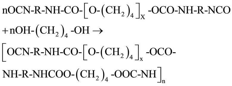
TPUs, which constitute the subject of this study, are linear polymers in which the principal chain structure is composed by two sections R1 and R2 connected via polar urethane groups (~R1-NH-COO-R2~). In this context, R1 denotes an aliphatic, aromatic or alicyclic radical derived from the isocyanate monomer while R2 denotes a more complex group derived from the polyol component (polyether or polyester). TPUs are typically obtained via a stepwise, polyaddition reaction between diisocyanates and bi-functional polyols with hydroxyl terminal groups, according to the following general scheme:
 (1)
(1)
It must also be noted that TPU chains do not contain only urethane structures. Depending on the specifications of feeds and on the method adopted for the polyaddition process, one can also find urea groups, biuret groups, allophanate groups, carbodiimide groups, aromatic hydrocarbon rings, isocyanurate or oxazolidone structures, and even ionic groups in some cases.
As a result of their physical and mechanical properties, associated to their good stability, low free surface energy, physiological inertness to living organisms and resistance to biodegradation, specialty TPUs are widely used as biomedical materials [11,12] capable of preventing inflammation of tissues, destruction by body fluids and deposition of blood components [13-16].
In most industrial cases, they are manufactured using traditional discontinuous processes which often give rise, from batch to batch, to products with inconstant quality.
The aim of the present work will be to develop and optimize a continuous process able to produce linear, solvent free and pure TPUs with controlled structure and specific end-use properties making them appropriate for on-line processing medical probes, catheters, cardiac valves and vascular prosthetic and endoprosthetic devices. In such case, reactive extrusion presents significant advantages as it can be used under well controlled operating conditions (feed rate, temperature, mixing rate, etc.).
This technique has already been widely exploited for the synthesis [17-22], grafting [23], hydrolysis [24] and depolymerization of TPUs [25], as well as for the production of oligomers [26]. However, in most cases, all the reactants were introduced into the extrusion machine in a single stage.
In the present study, we propose to elaborate TPUs in a two-stage process:
• First, a prepolymer will be synthesized in a batch reactor through catalyzed reactions between a macrodiol and a diisocyanate;
• The resulting prepolymer and a chain extender will then be introduced, under controlled operating conditions, into a twin-screw extruder to elaborate TPU chains.
It is expected that this procedure will contribute to the production of homogeneous TPUs with constant quality.
This work will start with a preliminary study devoted to determine the operating parameters for which the polymerization time and the average residence time of the reactants in the extruder must be of the same order of magnitude.
Then, an experimental strategy will be developed to study and model the effect of the extrusion parameters on the properties and the purity of the resulting TPUs.
The final objective will be to find a set of optimal operating conditions for the production, with the lowest energy consumption, of TPUs with targeted properties and high purity.
Accordingly, this optimization will be confronted with a multiobjective decision problem for which a unique solution that yields optimal values for all the objective criteria rarely exists. This is a common scenario in many industrial production optimizations which dictates the implementation of a decision-maker, in order to choose the best tradeoffs among all defined and conflicting objectives.
The methodology that will be used in this work has already been successfully applied to different polymerization processes [27-32]. It will be briefly described in the next section, while its specific application to this process will be discussed later.
2. Multicriteria Optimization Methodology
2.1. General Considerations
To develop industrial processes, companies need to obtain the desired products quality associated to the highest productivity and to the lowest cost investments. To reach these objectives, a multicriteria optimization of the process is necessary. In engineering processes, multiple objectives have usually been combined, often through linear [33] or empirical [34] combination, to form a scalar objective function. Another classical method consists in optimizing one criterion and setting up constraints on the others [35]. These techniques depend on the first user’s choice, so preferences can bias the result.
Methods incorporating a domination criterion are often more interesting because they are more general, more accurate and without any a priori knowledge. The aim is to find a non dominated zone in which a decision maker will be able to choose the best solution. This region, called Pareto’s zone, is the set of all non dominated points. It can be obtained using Pareto’s domination concept which is defined in such manner that a solution (compromise or vector), x1, dominates another solution, x2, if it is better or equal for all criteria and strictly better for at least one criterion [36]. The study does not allow to find immediately the preferred solution but to exclude all conditions which are not interesting. Two terms are used: Pareto’s domain and Pareto’s front which are related to the input variables and output criteria respectively.
Pareto’s domain can be approximated by a large number of possible solutions using an evolutionary algorithm [27,36-42]. It constitutes important information for the industrialist who will then have to classify these solutions.
Multiobjective optimization is commonly realized in a three-step procedure:
• Modelling of the process to encapsulate the underlying phenomena that relate all input and output process variables;
• Reduction of the decision space to include only the non-dominated solutions, providing an approximation of Pareto’s domain, using evolutionary algorithms;
• Ranking of all the solutions contained in Pareto’s domain using preferences from a human expert in order to choose the best compromise.
The most difficult step is usually the third one as it relates to a human-centred process that exhibits, by nature, a higher level of fuzziness. As a consequence, it is necessary to develop systematic procedures to unequivocally capture the preferences of the expert on the basis of his knowledge of the process.
In this respect, all the output criteria could be viewed as particular objective functions that need to be optimized. However, some of them are conflicting, making the optimization task significantly more difficult.
2.2. Methods for Ranking the Non-Dominated Solutions
A number of different methods have been proposed in the literature for performing the ranking procedure. In the present work, two methods will be used and compared, namely the “Net Flow” and the “Rough Set” methods. The main difference between these methods relies on the way the preferences of the experts are captured and used to determine the optimal zone of operation. It must be noted that it is not the objective of this study to detail these well-established methods, but rather to test, for this specific problem, whether convergent results can be obtained using them.
2.2.1. Net Flow Method (NFM)
NFM is a hybrid of two outranking methods (ELECTRE and PROMETHEE). It uses the knowledge of the objective criteria values and compares all non-dominated solutions, in a pairwise manner, to show a possible outranking before a total synthesis of the alternatives.
The user has to express several parameters to define his preferences.
First he must introduce a weight, wk, for each criterion k which serves as index of its relative importance. In the algorithm, these coefficients are normalized:
 (2)
(2)
The decision maker has also to define indifference, qk, preference, pk, and veto, vk, thresholds for each criterion. The indifference threshold is defined so that two alternatives cannot be differentiated below it. The preference threshold is defined to show the real preference of one alternative against another while the veto threshold is defined like a constraint if an alternative is too bad in one criterion. In this respect, an alternative is penalized if one of its criteria is over the veto threshold compared to another alternative, even if it is considered as a good alternative for the other criteria. Accordingly, these three thresholds are defined, for each criterion, in such a way that:
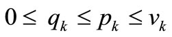 (3)
(3)
The criteria difference for each pair of alternatives, [i, j], and for each criterion, k, is:
 (4)
(4)
for ,
,  ,
,  and
and , and where fk(i) is the value of the kth criterion of alternative i, and hk is an optimization indicator (hk = 1 if fk is to be maximized and hk = −1 if fk is to be minimized).
A global concordance index, C[i, j], is then calculated as with ELECTRE III for each pair of alternatives (for i = 1, ∙∙∙, m and j = 1, ∙∙∙, m) [43].
The preference of one alternative over another is named “concordant” up to the indifference threshold and the local concordance index is then equal to 1. On the contrary, this preference is named “not concordant” up to the preference threshold and the local concordance index is then equal to 0. Between these two thresholds, a linear approach is used again to define the local concordance index:
 (5)
(5)
where
 (6)
(6)
A discordance index Dk[i, j] is also calculated for each criterion, k, as with ELECTRE III, to take into account a bad criterion value which allows to relegate the concerned point in the total ranking (for i = 1, ∙∙∙, m, j = 1, ∙∙∙, m and k = 1, ∙∙∙, n):
 (7)
(7)
The preference of an alternative versus another is called “discordant” up to the veto threshold and the discordance index is then equal to 1. On the contrary, it is named “not discordant” up to the preference threshold and the discordance index is then equal to 0. Between these two thresholds, a linear approach is used to define the discordance index.
Using the concordance and the discordance indexes, outranking degrees, σ[i, j], can be generated for every pair of alternatives. These outranking degrees are obtained using the following formula (for i = 1, ∙∙∙, m, j = 1, ∙∙∙, m) [44]:
 (8)
(8)
i outranks j all the more than the outranking degree is close to 1 .
.
The resulting outranking relation sets may be formulated in the form of an outranking matrix. From these outranking degrees, two preorders are established, as with PROMETHEE, by the outgoing flow  and the incoming flow
  (for i = 1, ∙∙∙, m) [45].
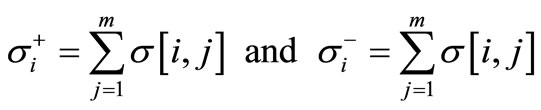 (9)
(9)
Finally, the total ranking of the alternatives, i, is determined from the net flow with possible ex æquo (for i = 1, ∙∙∙, m):
 (10)
(10)
The alternative, with the highest net flow, is considered as the “best” solution, while the one with the lowest net flow is considered as the “worst” solution, also known as “nadir”.
2.2.2. Rough Sets Method (RSM)
RSM is based on the Rough Set theory originally introduced by Pawlack [46-48] for ranking a large number of feasible solutions from Pareto’s zone. It has been used in several applications [49-54].
The classification of the compromises constitutes a “measurement” of the decision maker’s preference. A human expert classifies a small number of significant alternatives of Pareto’s Domain, in a preference descending order. Decision rules are then extracted in the form of a binary code (bits), thus creating a form of expert system. This decision-maker profile of preferences is subsequently applied to all the compromises. This allows different preference zones to be established.
The Rough Set theory uses a tabular representation of the preferential information expressed by the decision maker. The lines of this table correspond to objects whereas its columns correspond to attributes.
In the present study, the resulting table will be similar to the one suggested by Greco et al. [55]. More explanations will be given in Section 4.2.4.
In the original theory of Rough Sets, the rough approximations were performed using an indiscernibility relation on the pairwise comparison table. These approximations might result in inconsistencies between the generated rules, as discussed by Greco et al. [51]. To overcome this imprecision drawback, a different set of inconsistency rules [56] (Zaras (2001)) will be used in the present work. Finally, the finite set of solutions, representing the entire Pareto’s front, will be ranked by order of preference.
To achieve this classification, the Rough Sets Method uses the following steps:
• A small number of solutions (between 5 and 10) from different regions of Pareto’s zone are selected and presented to the expert who must classify them in a preference descending order (preferences measurement);
• Pairwise comparison of the solutions enables the extraction and validation of the “preference/no preference” rules, according to the RSM;
• These rules are subsequently applied to all the compromises, using the following principle: when two compared solutions are in accordance with a preference rule, then (+1) is added to the score of the first solution and (−1) is added to the score of the second solution;
• Finally, the resulting solutions are ranked in a scoredecreasing order.
3. Materials and Methods
3.1. Chemical Products and Reactions
Polyurethanes were synthesized using the products given in Table 1.
The first stage of the process was carried out by reaction between HMDI and PTMG to obtain the prepolymer (DI), made up of a flexible segment (PTMG) bearing one isocyanate function at each end. The corresponding reaction scheme is:
 (11)
(11)
With R: -(C6H10-CH2-C6H10)-.
In the second stage, the two isocyanate functions of DI reacted with the chain extender (EX) to give a blockpolyurethane composed of flexible segments alternating with the rigid ones. The chain extension took place according to the following reaction scheme:
 (12)
(12)
The prepolymerization was carried out in the presence of a catalyst, (dibutyltin dilaurate: DBTDL), which remained present and active during the chains extension stage as well. DBTDL concentration was 1 w% compared to the initial reactional mixture of PTMG and HMDI. Stoechiometry between HMDI, PTMG and EX was 2:1:2.
PTMG was used above its melting temperature (33˚C - 36˚C). Three PTMG were used with respective number average molar masses: MPTMG = 1000, 1400 and 2000 g/mol.
3.2. Reactors and Their Environment
Two batch reactors were used to develop the preliminary

Table 1. Main physical characteristics of the reagents.
studies:
Reactor 1 (i.e., the prepolymerization reactor) was a 200 mL jacketed glass batch reactor equipped with a stirrer, a reflux condenser, a cryostat, a sampling device and a nitrogen-supply system. The stirrer used was composed of a pitch blade turbine. Its rotation speed was kept constant at 500 rpm.
Reactor 2 was a Haake Rheocord-Rheomix internal mixer 540 p, equipped with a device which makes it possible to follow the time evolution of the torque and the temperature of the molten product.
It was composed of a basic device (Rheocord RC300 p) and a measuring cell (Rheomix R540 p). The whole system was controlled by a computer interface between the basic apparatus and the mixer, which was composed of a chamber with two rotating propeller-shaped rotors. The volume of this chamber was 50 mL, limited by a stop valve driven by a piston. The back wall, the intermediate room and the frontal plate were heated electrically and were equipped with independent control loops. A thermocouple, placed on the frontal plate of the mixer, measured the matter temperature. Cooling was achieved via channels crossed by compressed air and placed in the intermediate zone.
A Pilot unit for the chains extension was designed. It was composed of:
A prepolymerization batch reactor and its environment which includes 1) a tank for the storage of HMDI, equipped with a drainage sluice and a centrifugal pump, 2) a double-walled tank for the storage of PTMG, connected to a thermostat, an agitator, a drainage sluice and a gear pump, 3) a 15 liters capacity reactor, equipped with an agitator, feeding devices for HMDI, PTMG and the catalyst, a drainage sluice, a gear pump and temperature sensors, 4) an automat allowing to control the temperature and the feed rates of the reagents. Another tank was also available to store the solvent (Tetrahydrofuran) which was used for the cleaning of the two tanks and the reactor.
A corotative twin-screw-extruder (CLEXTRAL, BC21), equipped with interpenetrated screws and connected to the prepolymerization reactor via a gear pump and a flow-meter.
The extruder was also connected to a tank containing the chain extender via an HPLC pump.
The screws profile was determined so as to obtain a good mixture of the prepolymer and the chain extender and to maximize the residence time in the extruder, this in order to obtain the highest conversion. This profile included four elements of transport to quickly transport the prepolymer and the chain extender to the first zone of mixture, a regular alternation of elements of transport, elements with inversed steps and elements of mixing of variable steps and lengths. These last two types of elements allowed the formation of a pressure zone. The product accumulated in the threads of the upstream transport screws, thus increasing the rate of filling of the extruder and consequently the residence time of the reacting mixture.
The temperature control of the extruder barrel was achieved by means of electrical resistances and water circulation in the jacket of each constitutive element of the barrel, thus making it possible to establish the desired temperature profile along the barrel.
3.3. Analytical Methods
3.3.1. Number and Weight Average Molar Masses
The number and weight average molar masses were determined by size exclusion chromatography (SEC), using two detectors: a multi-angle laser light scattering (MALLS) apparatus (Dawn DSP-F) and a differential refractometer (Waters 410, Millipore).
Elutions were performed at 35˚C with tetrahydrofuran (THF) containing di-tertiary-butyl-2.6 methyl-4 phenol as stabilizer. The flow-rate was 1 mL∙min−1. The concentration of the polymer solutions and the corresponding injected volume were 1 g/L and 25 µL respectively. Prior to chromatography, THF and polymer solutions were passed through a Nylon filter of 0.45 µm porosity.
The SEC assembly consisted of a degasser, a Waters 510 Millipore pump, a U6K Millipore injector, a precolumn, two chromatographic columns assembled in series and filled with linear ultrastyragel and an electric oven to control the temperature of the columns. Data from the two detectors were acquired and exploited by means of the software Astra from Wyatt Technology which allowed the determination of the molar mass distribution and the number and weight average molar masses of the samples.
3.3.2. Residual Yield of Prepolymer (TDI)
TDI is given by:
 (13)
(13)
With:
 : TPUs number average molar mass;
MDI = 2 (MHMDI) + MPTMG + 2(MEX) = 705 + MPTMG where: MPTMG is 1000, 1400 or 2000 g/mol.
3.3.3. Glass Transition Temperature and Young’s Moduli
The glass transition temperature, Tg, as well as the temperature evolution of Young’s modulus, were obtained by dynamic mechanical thermal analysis, using the tensile testing machine DMTA V 902-50010 of Rheometric Scientific. This apparatus was coupled with a computer equipped with Orchestrator software which provided instantaneously the values of the shear storage modulus and loss modulus. Moreover, the apparatus was used in the “autostrain” mode, i.e. the imposed sinusoidal deformation was automatically adapted so that the measured stress remained higher than the sensitivity of the sensors. The initial distance between the jaws of the tensile testing machine was fixed at 6 mm.
Measurements were carried out on rectangular samples of 20 mm length, 13 mm of width and 2 mm of thickness which were obtained by using a manual hydraulic press. The operating conditions were the following:
• Test in three points.
• Frequency: 10 Hz.
• Constant deformation (0.1%).
• Temperature range: between −100˚C and +80˚C.
• Temperature rise speed: 3˚C∙min−1.
From the acquired data, the ratio of Young’s moduli, determined at Tg − 20˚C and Tg + 20˚C was subsequently calculated.
4. Results and Discussion
4.1. Preliminary Study
A preliminary study was carried out, in batch reactors and with moderate quantities of reagents, in order to define the operating conditions (temperature, catalyst concentration and mixing speed) which could be used to develop the continuous extrusion process. The first part of this study was focused on the kinetic modeling of the prepolymer synthesis while, the second part, dealt with the evaluation of the reaction time of the chains extension and the feasibility of the overall process.
4.1.1. Kinetic Model of the Prepolymer Synthesis
Initially, a set of experiments were carried out under the following operating conditions:
• Temperature: 100˚C.
• PTMG: 90.875 g.
• HMDI: 34.125 g.
• Catalyst: 3 different concentrations: 0.001 w%, 0.01 w% and 0.1 w%.
Samples were taken out at various reaction times and the weight concentration of unreacted isocyanate (NCO functional groups) was determined by a back-titration [57] (Otey et al., 1964).
The corresponding experimental data were subsequently used for the construction and the validation of a mathematical model of the prepolymerization kinetics which, in addition to the primary reaction given in scheme (11), considered also:
• One of the most important secondary reactions between urethane and isocyanate functional groups, which takes place after a certain conversion and results to the formation of allophanates, according to the following simplified mechanism: ![]()
 (14)
(14)
• The influence of the catalyst concentration on the reaction kinetics.
The rate of consumption of isocyanate functional groups was expressed by the following equation:
 (15)
(15)
where k1 and k2 are the rate constants of the primary and secondary reactions respectively. The technique of the minimum squared deviation between experimental and theoretical values was used to determine the values of these rate constants.
The results showed that:
• k1 depends on the catalyst concentration according to the following relation:
 (16)
(16)
and,
• k2 is constant and equal to 9.45 × 10⁻³ (kg/mol/s).
Figure 1 depicts the time evolution of NCO-groups conversion for the 3 catalyst concentrations and demonstrates:
• The good agreement between simulated and experimental data;
• That at 100˚C, the maximum conversion is obtained after around 180, 900 and 1100 seconds with 0.1, 0.01 and 0.001 w% catalyst concentration respectively.
4.1.2. Study of the Overall Process Using Haake Internal Mixer
The overall polymerization was carried out according to the following procedure:
In a first step, PTMG and HMDI were introduced in the mixing chamber and heated at 100˚C. The catalyst was then introduced (at a concentration of 0.1%). After 10 minutes of reaction, which exceeds the maximum time required to achieve the prepolymer synthesis, the temperature was raised to 160˚C and the chain extender was subsequently added.
The mixing speed of the first stage varied at each run from 5 to 200 rpm while that of the second stage was fixed at 160 rpm. The mixing torque was continuously recorded. During the reaction, the molar mass of the resulting TPU increased thus increasing the viscosity of the mixture as well. Hence, the mixing torque served as an indirect measurement of the progress of the reaction.
Figure 2 illustrates this interesting aspect showing clearly three distinct domains. In the first one, the value

Figure 1. Prepolymerization in the batch reactor: timeevolution of NCO-groups conversion for different catalyst concentrations.

Figure 2. Synthesis of TPUs using Haake internal mixer: time-evolution of the torque for different prepolymerization rotation speeds.
of the torque is near zero because of the low viscosity of the mixture. After the introduction of the chain extender, the curve exhibits a sharp peak due to a sudden increase of viscosity corresponding to the formation of chains with high molar masses.
After about five minutes, the reaction is complete and the torque reaches a constant value. A dependence of this constant value with the mixing speed used during the prepolymerization stage is clearly observed. This is probably due to a better mixing using the higher mixing speed which can improve the conversion during the first stage and, consequently, the production of more prepolymer molecules, i.e. in fine more final TPU chains during the second stage, thus inducing the higher viscosity of the final product.
Moreover, as shown in Table 2, the corresponding values of the weight average molar masses of the ten final products were similar ( ~175,000 g∙mol−1).
4.2. Reactive Extrusion Process
4.2.1. Operating Conditions
First stage: prepolymerization
This stage was carried out in the batch reactor of the pilot unit according to the following procedure:
• Heating (40˚C - 45˚C), vacuum drying of PTMG in order to eliminate traces of water and vacuum drying of HMDI.
• Circulation of a dry nitrogen current in PTMG and HMDI tanks and introduction of these two reagents into the reactor via transfer pumps. The introduced quantities were controlled by the transmitters of flow whose acquisition and integration of the signals on computer allowed the follow-up of the volumes and the stop of filling when the necessary quantities were reached.
• Homogenization and heating (55˚C) of the reacting

Table 2. Influence of the mixing speed used during the prepolymerization on the weight average molar masses of the TPUs. (Catalyst: 0.1 w%; Reaction time: First stage: 11 min; Second stage: 30 min; Reaction temperature: First stage: 100˚C; Second stage: 160˚C).
mixture followed by the injection of the catalyst.
• Maintenance under nitrogen and temperature control of the reaction medium at 90˚C. The reaction being very exothermic, the released thermal load (approximately 5 kW) could not be easily controlled. The reaction was thus carried out in a quasi adiabatic way.
• The standard operating conditions for the preparation of 10 kg of prepolymer were: MPTMG = 7.922 kg, MHMDI = 2.078 kg and MDBTDL = 10 g (w 0.1%).
Second stage: chains extension
The prepolymer was introduced at the feeding hopper of the extruder using the gear pump. Using the HPLC pump, the chain extender was introduced into the extruder using a liquid injector placed on one side of the elements of the barrel.
4.2.2. Experimental Strategy
On the basis of a factorial experimental design, 106 runs were carried out. For each run, the polyurethane samples were recovered at the outlet side of the die and analyzed in order to determine their number and weight average molar masses,  and
and , their glass transition temperature, Tg, and their Young’s modulus, ET, evolution with temperature. Additional measurements, useful for the process optimization, were also carried out during each run: the power necessary to ensure the rotation of the screws, W, and the pressure at the head of the die.
The input and output variables of the process and their operating range and target values are given in Table 3.
The input variables are the barrel temperature, T, the screws rotation speed, N, the prepolymer feed rate, Q,

Table 3. Input and output process variables.
and PTMG molar mass, MPTMG.
In this table:
• The energy consumption, E, is given by:
 (17)
(17)
where S, Troom and h are the heat-transferring surface, the room temperature, and the coefficient of heat exchange, respectively.
• The ratio, rE, is equal to:
 (18)
(18)
This expression is a simplification of the slope, STG, of a plot of Young’s modulus versus temperature:
 (19)
(19)
• The residual isocyanate yield, TDI, is given by Equation (13).
Figures 3 and 4, respectively, show the variations of  and Tg versus the screw rotation speed (N) for different prepolymer flow rates (Q) and barrel temperatures (T), of a polyurethane obtained using PTMG with a molar mass of 1400 g/mol.
These figures show that up to ~150 rpm,  and Tg vary only moderately as (N) increases. On the other hand, as expected for polycondensation reactions,
  increases, while Tg decreases as (T) and (Q) increase.

Figure 3. Synthesis of TPUs using Haake internal mixer: weight average molar mass versus screw rotation speed for different barrel temperatures and prepolymer flow-rates.

Figure 4. Synthesis of TPUs using Haake internal mixer: glass transition temperature versus screw rotation speed for different barrel temperatures and prepolymer flowrates.
4.2.3. Process Modelling
As already mentioned, prior to performing the optimization process, it is necessary to develop an adequate model capable of providing accurate predictions of all the principal outlet variables ( , TDI, Tg, rE, E), within the range of the considered operating conditions.
A deterministic model would require writing the mass and heat transfer equations coupled with the hydrodynamics in the extruder. This approach commonly leads to a complex algebraic-differential equation system which could not be easily usable in multicriteria optimization. Hence, a three-layer feedforward neural network (multilayer perceptron) was considered, using the quasi-Newton learning algorithm [58], to model each objective output variable of the process.
So, five models using the four input variables (T, N, Q, MPTMG) and able to calculate the values of the five output variables were established. The identification of the unknown parameters of these models required 76 runs, while 30 runs were used for the validation of the models. Moreover, for each network the number of neurons has been optimized in a range from 2 to 12, in order to avoid an over parameterization.
Table 4 indicates the number of neurons of the hidden layer corresponding to each outlet variable.
Figures 5-7 display a comparison between the simulated and experimental values of , E and rE, respectively. They clearly show that the models are able to predict with acceptable accuracy the output process variables.
4.2.4. Multicretiria Optimization and Decision Aid
Pareto’s domain approximation
Five objective criteria were determined on the basis of the five outputs of the models. They were divided to two process criteria, namely
- an energy criterion,
 (20)
(20)
- and a purity criterion,
 (21)
(21)
and to three quality criteria, defined by the following relationships:
 (22)
(22)
 (23)
(23)
 (24)
(24)
where,  ,
,  and
and  are target (desired) property values, depending on the particular use of the material. In the present study, these target values were selected on the basis of a commercial TPU named Tecoflex, which is marketed for medical use by Thermedics Polymer Products. They were equal to 63,000 g∙mol−1, −45˚C and 12.5, respectively.
The values of the four input variables were chosen randomly (initialization) and by a crossover operator in their operating range to generate, using the neural network models, the five output variables which, in turn, provided the corresponding five objective criteria (Equations (20)-(24)). The operating ranges of the experimental

Table 4. Number of neurons of the hidden layer of the neural network models.

Figure 5. Synthesis of TPUs by reactive extrusion: comparison of simulated and experimental values of weight average molar masses.

Figure 6. Synthesis of TPUs by reactive extrusion: comparison of simulated and experimental values of the energy consumption.
design (Table 3) were slightly enlarged in order to enable the exploration around the bounds. Roughly 5000 compromises, representing a set of candidate operating conditions, were generated.
To visualize the 4-dimensional input space and the 5- dimensional output space, a projection onto a 2-dimensional space was used. The resulting graphical representation was not perfect since the effect of the other dimensions created confounding areas. However, it was sufficient to provide information about the preferred zone of operation as well as the robustness of the optimal point.
For instance, in the input space, the projection of MPTMG versus T (Figure 8(a)) showed that the 5000 nondominated solutions were grouped in two fairly condensed areas surrounded by a diffuse set of points. This

Figure 7. Synthesis of TPUs by reactive extrusion: comparison of simulated and experimental values of Young’s moduli ratios.
was also observed in all the other input-input projections (e.g. in figures 9 and 10).
In the present study, all the criteria had to be minimized. All the output vs output graphs showed that, for each projection, the minima of the two corresponding criteria could be reached simultaneously. This is clearly illustrated in the example shown in Figure 8(b) through the projection of CTg versus CTx.
The values of both input variables and criteria corresponding to the centers of these two regions (Table 5) are very different. Hence, a choice, based on the preferences of a decision-maker, is essential.
Ranking of Pareto’s efficient solutions
The two previously presented ranking methods are used for this operation. For reasons of clarity, the conditions of their implementation will be presented separately. Then the results obtained using each one will be analyzed and compared.
1) Ranking Using the Net Flow Method
The values of the four parameters (i.e., weights, wk, indifference, qk, preference, pk and veto, vk, thresholds), as proposed by an expert of the process, are given in Table 6.
The selection of a proper level for each threshold is not an easy task since it requires a good knowledge of the process. In the present work, a maximum value was initially assigned to the weight average molar mass, via Pareto’s zone. Next, the indifference threshold was given a random value between 0.1 of the target value and 0.01 of the maximum value. Subsequently, the preference threshold was set at 5 times the indifference threshold and the veto threshold at 4 times the preference threshold. Concerning the weights, emphasis was given on Young’s moduli ratio to account for the importance of the processability of the final TPUs.
 (a) (b)
Figure 8. Examples of projections corresponding to the space of operating conditions used for the synthesis of TPUs. (a) Pareto’s zone of inputs variables MPTMG and T and (b) Pareto’s front of criteria CTg and CTx.

Table 5. Operating conditions and criteria corresponding to the centers of the two distinct areas of Pareto’s domain.

Table 6. Weights and indifference, preference and veto thresholds for each criterion.
The Decision Support Shell, described in Section 2.2.1, was then applied to the non-dominated compromises of Pareto’s domain, in order to rank them according to the values of the parameters chosen in this example.
2) Ranking Using the Rough Sets Method (RSM)
The method described in Section 2.2.2 was used to obtain the preference or non-preference rules, which were applied to all the compromises of the previously obtained Pareto’s front.
Table 7 presents the resulting sets of rules, generated by the pair-wise comparison of ten alternatives, previously ranked by the decision maker. 45 such comparisons produced an equal number of candidate rules. Some were redundant while others were contradictory. After elimination of each redundant rule and of those being contradictory, 16 rules were preserved.
Considering two alternatives, A and B, to be ranked according to rule 1, the corresponding preference rule (00100) was expressed as:
IF CMw is worse for A than for B, AND CTx is worse for A than for B, AND CE is better for A than for B, AND CTg is worse for A than for B, AND CrE is worse for A. According to Section 2.2.2, (+1) is then attributed to B.
The corresponding non preference rule (11011) is expressed as:
IF CMw is better for A than for B, AND CTx is better for A than for B, AND CE is worse for A than for B, AND CTg is better for A than for B, AND CrE is better for A than for B, THEN B is not preferred over A. (−1) is then attributed to B.
Accordingly, in Table 7, (0) corresponds to “worse than” while (1) corresponds to “better than” or “equal to”.
Even though the method seems simplistic, a single rule cannot be interpreted without considering the complete set of rules. For example, it is impossible to infer, from rule 1, that only the criterion CE is relevant. In fact, overall criteria have the same importance in the sixteen rules (there are no associated weights).
These rules are an approximation of the choice process of the decision maker as a set, including its apparent inconsistencies. In fact, this process is often complex and cannot be reduced to a logical reasoning. This becomes
 (a) (b)
Figure 9. Ranking of the 10% best solutions (black points) and the overall best (white square) of Pareto’s zone corresponding to input variables Q and T using: (a) the net flow method and (b) the rough sets method.
 (a) (b)
Figure 10. Ranking of the 10% best solutions (black points) and the overall best (white square) of Pareto’s zone corresponding to input variables N and T using: (a) the net flow method and (b) the rough sets method.
apparent when attempting to compare, for example, rules #5 and #15. This is the main reason for the implementation of a method that is approximate and less precise than that of the assessments of the NFM, for modeling the process choice of the decision maker. The advantages of this method are its simplicity in application and computational speed.
3) Analysis and Comparison of the Results
Figures 9-12 display the projection of the results obtained by the application of these two ranking methods to:
• Q and T (Figures 9(a) and (b)) and N and T (Figures 10(a) and (b)).
• CTg and CrE (Figures 11(a) and (b)) and CE and CTx (Figures 12(a) and (b)).
Each Figure also displays the 10% best solutions as well as the overall best solution, represented by black points and by a white square, respectively.
All figures clearly show that the projections of the 10% best solutions, resulting from each ranking method, do not cover the same domain. Moreover, the points obtained using the RSM are more dispersed than those obtained using the NFM.
This confirms the lower degree of accuracy of the results obtained using the RSM.
Table 8 shows the best and worst values of the input process variables and corresponding criteria obtained using the Net Flow and Rough Sets Methods.
To validate these results, two experimental runs were carried out using the operating conditions presented in Table 9. As PTMG samples, with molar masses equal to those preferred by the two ranking methods (i.e., 1805 and 2100 kg/kmol), were not available for this validation, the two experiments were carried out using PTMG with a molar mass of 2000 kg/kmol. All the remaining experimental conditions were kept as close as possible to the optimal ones, indicated by each ranking method.
The resulting criteria values, also given in Table 9, clearly show that the best experimental results are close to those obtained using the NFM, thus confirming the

Table 7. Set of rules generated by use of the rough sets method.
 (a) (b)
Figure 11. Ranking of the 10% best solutions (black points) and the overall best (white square) of Pareto’s front corresponding to criteria CTg and CrE using: (a) the net flow method and (b) the rough sets method.
superior performance of this ranking method, without rejecting, at the same time, the values obtained using the RSM. Due to the nature of RSM, the preferred point shows two criteria that are not well predicted by the neural network simulators, i.e. the power consumption, whose predicted value is 1.15 kJ/kg while the two experimental values are 10.4 and 13.5 kJ/kg, and the glass transition temperature, whose predicted value is 2.6˚C while the two experimental values are 0.25˚C and 0.10˚C. However, these differences remain within the range of the model uncertainty.
This analysis clearly shows that the two ranking methods implemented in this work provide similar, but not strictly identical, results.
 (a) (b)
Figure 12. Ranking of the 10% best solutions (black points) and the overall best (white square) of Pareto’s front corresponding to criteria CE and CTx using: (a) the net flow method and (b) the rough sets method.
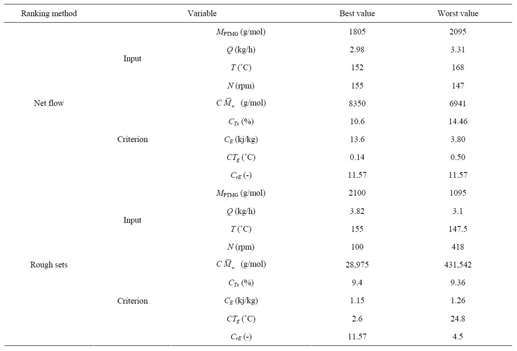
Table 8. Best and worst values of the input process variables and corresponding criteria obtained using the net flow and rough sets methods.
5. Conclusions
The present work concerns the optimization of a reactive extrusion process for the synthesis of linear thermoplastic polyurethanes adapted to medical uses.
The experiments were carried out under bulk conditions which present undeniable advantages in terms of safety and protection of the environment. The absence of solvent allows avoiding eventual stages of purification of the final product and recycling of the solvent. In addition the maintenance and cleaning operations, which are necessary after each batch run, are simplified. Moreover, compared to batch or semi-batch processes, this con-

Table 9. Comparison between the best solutions (input variables and criteria) obtained using the net flow and rough sets methods and the experimental values.
tinuous process allows, once the optimized operating conditions and the stationary state are reached, obtaining with a higher rate of production, materials with more homogeneous properties. In addition, in the present case, the synthesis can be integrated into the on-line manufacture of specific final products (e.g., catheters, implants, etc.). This will result in an appreciable time-saver which will be reflected on the overall costs of the process.
Hence, a multicriteria optimization of the process apared to be of profound interest. To develop the optimization strategy, a two-stage process was developed.
A preliminary study allowed determining the process operating conditions for which the polymerization time and the average residence time of the reactants in the extruder were of the same order of magnitude. This was done through a series of experiments which allowed:
• Determining, owing to the elaboration of a kinetic model, the optimal experimental conditions (temperature and catalyst concentration) of the first stage;
• Showing, through a study of the overall process using a Haake internal mixer, that after about five minutes, the polymerization could be complete.
The extrusion process was then developed using a factorial experimental strategy which allowed studying the influence of the input process variables (T, N, Q, MPTMG), on a number of selected outputs, which include the TPU production yield, the energy consumption (E), the main properties of the polyurethanes ( , Tg, rE,) and their purity (TDI).
This information was subsequently used to construct neural models which were able to predict, with acceptable accuracy, the output variables of the process.
These models were, in turn, used to determine, with the help of an evolutionary algorithm, a series of 5000 non-dominated alternatives, constituting Pareto’s domain.
The multicriteria analysis of this set of compromises was finally carried out using two methods, namely the Net Flow and the Rough Sets Methods which, taking into account the preferences of a decision maker, allowed the ranking of the Pareto’s zone alternatives. NFM develops a powerful mathematical approach, whereas RSM provides an approximate decision model which includes possible contradictions of the decision maker but whose implementation is simple with rather short computing times.
These two methods made it possible to propose acceptable recommendations for the operating conditions of the process. Experimental validation runs carried out under similar operating conditions gave rise to criteria values confirming the superior performance of NFM, without rejecting, at the same time, the values obtained using RSM.
6. Acknowledgements
The authors are grateful to the French Ministry of Education and Research and to the Lorraine Regional Council for their financial support.
REFERENCES
- P. Król, “Synthesis Methods, Chemical Structures and Phase Structures of Linear Polyurethanes. Properties and Applications of Linear Polyurethanes in Polyurethane Elastomers, Copolymers and Ionomers,” Progress in Materials Science, Vol. 52, No. 6, 2007, pp. 915-1015. doi:10.1016/j.pmatsci.2006.11.001
- J. M. Raqueza, M. Deléglisea, M. F. Lacrampea and P. Krawczaka, “Thermosetting (Bio)materials Derived from Renewable Resources: A Critical Review,” Progress in Polymer Science, Vol. 35, No. 4, 2010, pp. 487-509. doi:10.1016/j.progpolymsci.2010.01.001
- P. F. Brains, “Polyurethanes Technology,” John Wiley & Sons, Hoboken, 1969.
- C. Hepburn, “Polyurethane Elastomers,” Elsevier Science, London, 1992. doi:10.1007/978-94-011-2924-4
- Z. Wirpsza, “Polyurethane, Chemistry, Technology and Applications,” Ellis Harwood, Chichester, 1993.
- J. Dodge, “Polyurethane Chemistry,” 2nd Edition, Bayer Corp., Pittsburgh, 1999.
- D. K. Chattopadhyay and K. V. Raju, “Structural Engineering of Polyurethane Coatings for High Performance Applications,” Progress in Polymer Science, Vol. 32, No. 3, 2007, pp. 352-418. doi:10.1016/j.progpolymsci.2006.05.003
- R. Narayan, D. K. Chattopadhyay, B. Sreedhar, K. V. Raju, N. N. Mallikarjuna and T. M. Aminabhavi, “Synthesis and Characterization of Cross-Linked Polyurethane Dispersions Based on Hydroxylated Polyesters,” Journal of Applied Polymer Science, Vol. 99, No. 1, 2006, pp. 368-380. doi:10.1002/app.22430
- A. A. Caraculacu and S. Coseri, “Isocyanates in Polyaddition Processes, Structure and Reaction Mechanisms,” Progress in Polymer Science, Vol. 26, No. 5, 2001, pp. 799-851. doi:10.1016/S0079-6700(00)00033-2
- K. M. Zia, H. N. Bhatti and I. A. Bhatti, “Methods for Polyurethane and Polyurethane Composites, Recycling and Recovery: A Review,” Reactive and Functional Polymers, Vol. 67, No. 8, 2007, pp. 675-692. doi:10.1016/j.reactfunctpolym.2007.05.004
- P. A. Gunatillake, D. J. Martin, G. F. Meijs, S. J. McCarthy and R. Adhikari, “Designing Biostable Polyurethane Elastomers for Biomedical Implants,” Australian Journal of Chemistry, Vol. 56, No. 6, 2003, pp. 545-557. doi:10.1071/CH02168
- J. H. Park, K. D. Park and Y. H. Bae, “PDMS Based Polyurethane Grafted with MPEG: Synthesis, Characterization and Platelet Adhesion Property,” Biomaterials, Vol. 20, No. 10, 1999, pp. 943-953. doi:10.1016/S0142-9612(98)00250-6
- L. Poussard, F. Burel, J. P. Couvercelle, Y. Merhi, M. Tabrizian and C. Bunel, “Haemocompatibility of New Ionic Polyurethanes. Influence of Carboxylic Group Insertion Modes,” Biomaterials, Vol. 25, No. 17, 2004, pp. 3473-3483. doi:10.1016/j.biomaterials.2003.10.069
- J. H. Wang and C. H. Yao, “Development of Biodegradable Polyester Urethane Membranes with Different Surface Morphologies for the Culture of Osteoblasts,” Journal of Biomedical Materials Research, Vol. 51, No. 4, 2000, pp. 761-769. doi:10.1002/1097-4636(20000915)51:4<761::AID-JBM26>3.0.CO;2-2
- K. Gorna and S. Gogolewski, “In Vitro Degradation of Novel Medical Biodegradable Aliphatic Polyurethanes Based on Epsilon-Caprolactone and Pluronics (R) with Various Hydrophilicities,” Polymer Degradation and Stability, Vol. 75, No. 1, 2002, pp. 113-122. doi:10.1016/S0141-3910(01)00210-5
- K. Gorna and S. Gogolewski, “Biodegradable Polyurethanes for Implants. II. In Vitro Degradation and Calcification of Materials from Poly(epsilon-caprolactone)-poly (ethylene oxide) Diols and Various Chain Extenders,” Journal of Biomedical Materials Research, Vol. 60, No. 4, 2002, pp. 592-606. doi:10.1002/jbm.10100
- R. M. Hensarling, J. G. Ruy, A. Hill and S. J. Moravek, “Twin Screw Extrusion: Formation of Thermoplastic Polyurethane through Reactive Extrusion,” American Chemical Society, Polymer Preprints, Division of Polymer Chemistry, Vol. 49, No. 1, 2008, pp. 1163-1164.
- S. J. Moravek, J. S. Wiggins and R. F. Storey, “Reactive Extrusion of Methyl 2,6-Diisocyantocaproate-Based Degradable Thermoplastic Polyurethanes,” American Chemical Society Polymer Preprints, Division of Polymer Chemistry, Vol. 49, No. 1, 2008, pp. 574-575.
- A. Lapprand, F. Méchin and J. P. Pascault, “Synthesis and Properties of Self-Crosslinkable Thermoplastic Polyurethanes,” Journal of Applied Polymer Science, Vol. 105, No. 1, 2007, pp. 99-113. doi:10.1002/app.26086
- J. P. Puaux, P. Cassagnau, G. Bozga and I. Nagy, “Modeling of Polyurethane Synthesis by Reactive Extrusion,” Chemical Engineering and Processing: Process Intensification, Vol. 45, No. 6, 2006, pp. 481-487. doi:10.1016/j.cep.2005.11.006
- A. Bouilloux, C. W. Makosco and T. Kotnour, “Urethane Polymerization in a Counterrotating Twin-Screw Extruder,” Industrial and Engineering Chemistry Research, Vol. 30, No. 11, 1991, pp. 2431-2436. doi:10.1021/ie00059a011
- M. E. Hyun and S. C. Kim, “A Study on the Reactive Extrusion Process of Polyurethane,” Polymer Engineering and Science, Vol. 28, No. 11, 1998, pp. 743-757. doi:10.1002/pen.760281107
- S. Dassin, M. Dumon, F. Mechin and J. P. Pascault, “Thermoplastic Polyurethanes (TPUs) with Grafted Organosilane Moieties: A New Way of Improving Thermomechanical Behavior,” Polymer Engineering and Science, Vol. 42, No. 8, 2002, pp. 1724-1739. doi:10.1002/pen.11066
- T. Taniguchi, N. Sato, M. Matsushita, H. Takahashi, T. Suzuki, Y. Hoshino and N. Abe, “Hydrolysis of Polyurethane Resin Using a Twin Screw Reactive Extruder for Recycle,” Kobunshi Ronbunshu, Vol. 56, No. 11, 1999, pp. 709-716. doi:10.1295/koron.56.709
- V. W. A. Verhoeven, A. D. Padsalgikar, K. J. Ganzeveld and L. P. B. M. Janssen, “The Reactive Extrusion of Thermoplastic Polyurethane and the Effect of the Depolymerization Reaction,” International Polymer Processing, Vol. 21, No. 3, 2006, pp. 295-308.
- J. Chen, J. P. Pascault and M. Taha, “Synthesis of Polyurethane Acrylate Oligomers Based on Polybutadiene Polyol,” Journal of Polymer Science, Part A: Polymer Chemistry, Vol. 34, No. 14, 1996, pp. 2889-2907. doi:10.1002/(SICI)1099-0518(199610)34:14<2889::AID-POLA6>3.0.CO;2-M
- S. Massebeuf, C. Fonteix, S. Hoppe and F. Pla, “Development of New Concepts for the Control of Polymerisation Processes: Multiobjective Optimization and Decision Engineering. Part I. Application to Emulsion Homopolymerization of Styrene,” Journal of Applied Polymer Science, Vol. 87, No. 14, 2003, pp. 2383-2396. doi:10.1002/app.12026
- C. Fonteix, S. Massebeuf, F. Pla and L. N. Kiss, “Multicriteria Optimization of an Emulsion Polymerization Process,” European Journal of Operational Research, Vol. 153, No. 2, 2004, pp. 350-359. doi:10.1016/S0377-2217(03)00157-7
- A. Nayak and S. K. Gupta, “Multiobjective Optimization of Semi-Batch Copolymerization Reactors Using Adaptations of Generic Algorithm,” Macromolecular Theory and Simulations, Vol. 13, No. 1, 2004, pp. 73-85. doi:10.1002/mats.200350033
- E. Ginsburger, “Définition et Mise au Point d’une Méthodologie pour L’extrapolation de Procédés de Copolymérisation,” Ph.D. Dissertation, University of Nancy, Lorraine, 2001.
- B. Benyahia, M. A. Latifi, C. Fonteix and F. Pla, “Multicriteria Dynamic Optimization of an Emulsion Copolymerization Reactor,” Computer Aided Chemical Engineering, Vol. 28, 2010, pp. 457-462. doi:10.1016/S1570-7946(10)28077-X
- F. Pla, R. Rached, S. Hoppe and C. Fonteix, “Design and Multiobjective Optimization of a Novel Reactive Extrusion Process for the Production of Nanostructured PA12/ PDMS Blends,” Proceedings of the Nanotech Conference and Expo IIFNBM, Anaheim, 21-25 June 2010, pp. 885- 888.
- P. Courcoux, E. M. Qannari, J. P. Melcion and J. Morat, “Optimisation Multiréponse: Application à un Procédé de Granulation D’aliments,” Récents Progrès en Génie des Procédés: Stratégie Expérimentale et Procédés Biotechnologiques, Vol. 36, No. 9, 1995, pp. 41-47.
- C. Azzaro-Pantel, L. Bernal-Haro, P. Baudet, S. Domenech and L. Pibouleau, “A Two-Stage Methodology for Short-Term Batch Plant Scheduling: Discrete-Event Simulation and Genetic Algorithm,” Computers & Chemical Engineering, Vol. 22, No. 10, 1998, pp. 1461-1481. doi:10.1016/S0098-1354(98)80033-1
- N. Logothetis and A. Haigh, “Characterizing and Optimizing Multi-Response Processes by the Taguchi Method,” Quality and Reliability Engineering International, Vol. 4, No. 2, 1988, pp. 159-169. doi:10.1002/qre.4680040211
- R. Viennet, C. Fonteix and I. Marc, “Multicriteria Optimization Using a Genetic Algorithm for Determining a Pareto Set,” International Journal of Systems Science, Vol. 27, No. 2, 1996, pp. 255-260. doi:10.1080/00207729608929211
- F. Bicking, C. Fonteix, J. P. Corriou and I. Marc, “Global Optimization by Artificial Life: A New Technique Using Genetic Population Evolution,” RAIRO-Operations Research, Vol. 28, No. 1, 1994, pp. 23-36.
- C. Fonteix, F. Bicking, E. Perrin and I. Marc, “Haploid and Diploid Algorithms: A New Approach for Global Optimization: Compared Performances,” International Journal of Systems Science, Vol. 26, No. 10, 1995, pp. 1919-1933. doi:10.1080/00207729508929145
- S. Shabeer and M. Y. Wang, “Multiobjective Optimization of Sequential Brake Forming Processes,” Journal of Materials Processing Technology, Vol. 102, No. 1-3, 2000, pp. 266-276. doi:10.1016/S0924-0136(00)00492-1
- V. Bhaskar, S. K. Gupta and A. K.Ray, “Multiobjective Optimization of an Industrial Wiped Film PolyethyleneTerephthalate Reactor: Some Further Insights,” Composites and Chemical Engineering, Vol. 25, No. 2-3, 2001, pp. 391-407. doi:10.1016/S0098-1354(00)00665-7
- H. Hamda, O. Roudenko and M. Schoenauer, “Application of a Multiobjective Evolutionary Algorithm to Topological Optimum Design,” In: I. Parmee, Ed., Adaptive Computing in Design and Manufacture, Springer-Verlag, London, 2002, pp. 121-132. doi:10.1007/978-0-85729-345-9_11
- L. Muniglia, L. N. Kiss, C. Fonteix and I. Marc, “Multicriteria Optimization of a Single-Cell Oil Production,” European Journal of Operational Research, Vol. 153, No. 2, 2004, pp. 360-369. doi:10.1016/S0377-2217(03)00158-9
- B. Roy, “ELECTRE III: Algorithme de Classement Basé sur une Représentation Floue des Préférences en Présence de Critères Multiples,” Cahiers du CERO, Vol. 20, No. 1, 1978, pp. 3-24.
- A. Rousseau and J. M. Martel, “Environmental Assessment of an Electric Transmission Line Project: A MCDA Method,” In: M. Paruccini, Ed., Applying Multiple Criteria Aid for Decisions to Environmental Management, Kluwer Academic Publishers, Dordrecht, 1994, pp. 163- 185.
- J. P. Brans and P. H. Vincke, “A Preference Ranking Organization Method: The PROMETHEE Method for Multiple Criteria Decision Making,” Management Science, Vol. 31, No. 6, 1985, pp. 647-656. doi:10.1287/mnsc.31.6.647
- Z. Pawlak, “Rough Sets,” Informational Journal of Information and Computer Sciences, Vol. 11, No. 5, 1982, pp. 341-356. doi:10.1007/BF01001956
- Z. Pawlak, “Rough Sets. Theoretical Aspects of Reasoning about Data,” Kluwer Academic Publishers, Dordrecht, 1991.
- Z. Pawlak, “Rough Set Approach to Knowledge-Based Decision Support,” European Journal of Operational Research, Vol. 99, No. 1, 1997, pp. 48-57. doi:10.1016/S0377-2217(96)00382-7
- J. Thibault, R. Lanouette, C. Fonteix and L. N. Kiss, “Multicriteria Optimization of an High Yield Pulping Process,” Canadian Journal of Chemical Engineering, Vol. 80, No. 5, 2002, pp. 897-902. doi:10.1002/cjce.5450800512
- M. Hapke, A. Jaszkiewicz and R. Slowinski, “Interactive Analysis of Multiple-Criteria Project Scheduling Problems,” European Journal of Operational Research, Vol. 107, No. 2, 1998, pp. 315-324. doi:10.1016/S0377-2217(97)00336-6
- S. Greco, B. Matarazzo and R. Slowinski, “Rough Sets Approximation of a Preference Relation by Dominance Relations,” European Journal of Operational Research, Vol. 117, No. 1, 1999, pp. 63-83. doi:10.1016/S0377-2217(98)00127-1
- S. Greco, B. Matarazzo and R. Slowinski, “The Use of Rough Sets and Fuzzy Sets in MCDM,” In: T. Gal, T. Stewart and T. Hanne, Eds., Advances in Multiple Criteria Decision Making, Kluwer Academic Publishers, Boston, 1999, pp. 1-14.
- S. Greco, B. Matarazzo and R. Slowinski, “Rough Sets Theory for Multicriteria Decision Analysis,” European Journal of Operational Research, Vol. 129, No. 1, 2001, pp. 1-47. doi:10.1016/S0377-2217(00)00167-3
- S. Greco, B. Matarazzo and R. Slowinski, “Rough Sets Methodology for Sorting Problems in Presence of Multiple Attributes and Criteria,” European Journal of Operational Research, Vol. 138, No. 2, 2002, pp. 247-259. doi:10.1016/S0377-2217(01)00244-2
- S. Greco, B. Matarazzo and R. Slowinski, “Rough Approximation of a Preference Relation in a Pairwise Comparison Table,” In: A. Skowron and L. Polkowski, Eds., Rough Sets in Knowledge Discovery, Physica-Verlag, Heidelberg, 1998.
- K. Zaras, “Rough Approximation of Preference Relation by a Multiattribute Stochastic Dominance for Deterministic and Stochastic Evaluation Problems,” European Journal of Operational Research, Vol. 130, No. 12, 2001, pp. 305-314. doi:10.1016/S0377-2217(00)00046-1
- F. H. Otey, B. L. Zagoren and C. L. Mehltretter, “Determination of Hydroxyl Number of Polyoxyalkylene Ethers by Reaction with Toluene Diisocyanate,” Journal of Applied Polymer Science, Vol. 8, 1964, pp. 1985-1989. doi:10.1002/app.1964.070080505
- R. Lanouette, J. Thibault and J. L. Valade, “Process Modeling with Neural Networks Using Small Experimental Datasets,” Computers and Chemical Engineering, Vol. 23, No. 9, 1999, pp. 1167-1176.
Notations
A: Alternative of Pareto’s zone
B: Alternative of Pareto’s zone
 : Global concordance Index
CMw (g/mol): Weight average molar mass criterion
CrE: Young’s modulus ratio criterion
CTg (˚C): Glass transition temperature criterion
CTx (%): Residual yield of DI criterion
DBTDL: Dibutyltin dilaurate
 : Discordance index
E (kj/kg): Energy consumption
ET (Pa): Young’s modulus
EX Chain extender: (1,4-butanediol) fk(i) value of the kth criterion of alternative i h (kW/m2/˚C) Coefficient of heat exchange
HMDI: Hexamethylene diisocyanate: (Methylene bis-4- cyclohexyl-isocyanate)
k1 (kg/mol/s): Rate constant of the primary reaction of the prepolymer synthesis
k2 (kg/mol/s): Rate constant of the secondary reaction of the prepolymer synthesis
MDI (g/mol): Prepolymer molar mass
 (g/mol): Number average molar mass
 (g/mol): Weight average molar mass
 (g/mol): Target value of the weight average molar mass
N (rpm): Screws rotation speed
NFM: Net Flow Method
pk: Preference threshold of criterion k
Q (kg/h): Prepolymer feed rate
R: Initial ratio of NCO to OH
rE: Young’s modulus ratio
 : Target value of Young’s modulus ratio
RSM: Rough Sets Method
S (m2): Heat-transferring surface
STG (Pa/˚C): Slope of a plot of Young’s modulus versus temperature
T (˚C): Temperature of the barrel
Troom (˚C): Room temperature
TDI (%): Residual yield of DI
Tg (˚C): Glass transition temperature
TgC (˚C): Target value of glass transition temperature
TPU: Thermoplastic polyurethane
w%: Concentrations (weight %)
W (kW): Power to ensure the rotation of the screws
wk: Weight of criterion k
Greek letters
 : Criteria difference for each pair of alternatives
[i, j] and each criterion k
hk: Optimization indicator
σ [i, j]: Outranking degrees for every pair of alternatives
 ,
, : Outgoing flow and incoming flow for NFM
vk: Veto threshold of criterion k