Sim-to-Real: A Performance Comparison of PPO, TD3, and SAC Reinforcement Learning Algorithms for Quadruped Walking Gait Generation

James W. Mock, Suresh S. Muknahallipatna^*

Department of Electrical Engineering and Computer Science, University of Wyoming, Laramie, WY, USA.

DOI: 10.4236/jilsa.2024.162003                

Abstract

The performance of the state-of-the-art Deep Reinforcement algorithms such as Proximal Policy Optimization, Twin Delayed Deep Deterministic Policy Gradient, and Soft Actor-Critic for generating a quadruped walking gait in a virtual environment was presented in previous research work titled “A Comparison of PPO, TD3, and SAC Reinforcement Algorithms for Quadruped Walking Gait Generation”. We demonstrated that the Soft Actor-Critic Reinforcement algorithm had the best performance generating the walking gait for a quadruped in certain instances of sensor configurations in the virtual environment. In this work, we present the performance analysis of the state-of-the-art Deep Reinforcement algorithms above for quadruped walking gait generation in a physical environment. The performance is determined in the physical environment by transfer learning augmented by real-time reinforcement learning for gait generation on a physical quadruped. The performance is analyzed on a quadruped equipped with a range of sensors such as position tracking using a stereo camera, contact sensing of each of the robot legs through force resistive sensors, and proprioceptive information of the robot body and legs using nine inertial measurement units. The performance comparison is presented using the metrics associated with the walking gait: average forward velocity (m/s), average forward velocity variance, average lateral velocity (m/s), average lateral velocity variance, and quaternion root mean square deviation. The strengths and weaknesses of each algorithm for the given task on the physical quadruped are discussed.

Keywords

Reinforcement Learning, Reality Gap, Position Tracking, Action Spaces, Domain Randomization

1. Introduction

The performance comparison of three state-of-the-art Reinforcement algorithms, namely the Proximal Policy Optimization (PPO), Twin Delayed Deep Deterministic Policy Gradient (TD3), and Soft Actor-Critic (SAC) for the walking gait of a quadruped robot were presented by the authors in their previous article [1] . The performance of the three algorithms was studied on a quadruped robot simulated by modeling the robot using MuJoCo’s native MJCF modeling language. Each algorithm’s performance was evaluated in seven different state spaces along with addressing the simulation optimization basis (domain randomization). The performance results demonstrated the performance of the three algorithms was dependent on the sensor configurations, i.e., the state space. However, the performance results of the three algorithms in the virtual environment did not present a clear winner. This paper compares the three algorithms’ performance in the physical environment or the real world by transfer learning on a real quadruped. This paper is organized as follows: Section 2 presents the techniques used to close the reality gap (RG) between the virtual and physical environments. The experimental setup discussions are presented in section 4. Section 5 presents the performance of the three algorithms on the quadruped in the physical environment. Section 6 presents the conclusions.

2. Methodologies for Solving RG

In most cases, training RL algorithms on real robots is impractical due to time considerations or the potential for damaging the robot. Therefore, RL algorithms are often trained in a simulated environment and transferred to the real robot. The reality gap remains the largest obstacle to using reinforcement learning for walking robots [2] . Most current research has been devoted to closing the reality gap through zero-shot transfer methods. Zero-shot methods are methods that perform all policy training in simulation. Once the training is complete, the trained policy is directly implemented on the physical robot [3] . These methods focus on modifying simulations so that trained policies can be directly deployed on a physical robot without any additional training or adjustments to the robot.

2.1. System Identification

The most common method used to close the reality gap is known as system identification. System identification refers to methods that modify simulated environments to make them more reflective of the real world. This is often done by hand modeling elements having the greatest impact on the learning, such as accurate physics and robot models. Accurate CAD models of a robot are often essential for successful real-world simulation deployment. A significant portion of development time is used to make the rigid body models used in the simulation. Xie et al. [4] ensured the mass and inertia of each link in a bipedal robot were accurate. Additionally, an accurate model of the motors’ reflected inertia, especially for the knee joints, was critical to successfully deploying a trained policy onto the physical robot. Despite improvements in physics simulators and CAD software, it is still impossible to perfectly replicate a physical robot in simulation. Researchers estimate there is still a significant error because electronics and cabling are usually not modeled [5] . Physical parameters that change due to temperature, humidity, positioning, and wear-and-tear further complicate system identification. Accurately reproducing the geometric properties of a robot is just one type of system identification. It has been shown that imitating real-world motor dynamics and latencies can also improve real-to-simulation transferability [5] [6] . For example, Tan et al. [6] successfully transferred a policy learned in the simulation to an under-actuated quadruped by accurately modeling the actuator dynamics and observation latency. The actuator model was based on ideal DC motor models. Latencies were simulated by using a linear interpolation of two prior consecutive observations. Latency times were measured on the real robot and then used to set the correct latency in the simulation. Some researchers have attempted to use supervised learning to match real-world dynamics to simulations. In Hwangbo et al. [5] , an Artificial Neural Network was used to approximate the real actuator dynamics and latencies in simulation. This allowed for a walking gait that outperformed the original classical controller regarding tracking error while using up to 36% less torque.

2.2. Domain Randomization

The inevitable imperfections of physics simulations will automatically be exploited by optimization methods if they help achieve an improvement. However, since these exploits don’t exist in the real world, policies transferred to the real world will not perform as expected. This is known as the simulation optimization bias (SOB) [7] . One method to combat SOB is to randomize the parameters of the simulation. Unlike system identification, which aims to model the real world carefully, domain randomization aims to randomize a simulation’s visuals or system dynamics to encourage generalization. System identification and domain randomization are often used to achieve better results [3] [5] [6] . Early domain randomization techniques largely added i.i.d. noise to observations and actions [7] . Newer techniques involve changing the appearance and core dynamics of a simulated environment. Vision-based learning has a particularly wide reality gap because it is difficult to generate high-quality, realistically rendered images [3] . Additionally, simulated cameras fail to incorporate noise and optical distortions produced by real cameras [8] . For vision-based object manipulation tasks, Pinto et al. [9] randomized textures, lighting, and the camera’s position. They found that policies trained without domain randomization failed to perform when transferred to the real robot. Parameters like mass, friction coefficients, and actuator behavior are randomized for non-vision-based robots. Tan et al. [6] found that using inertia randomization when learning a quadruped gait significantly improves robustness at the cost optimality. This means domain randomization causes the simulated policy to have degraded performance but will perform better on the physical robot. Adversarial disturbances to the agent are another common form of domain randomization. Rudin et al. [10] implemented this idea by pushing the simulated robot every 10 seconds. The robot’s base is accelerated up to ±1 m/s in both x and y directions. This results in a highly stable and dynamic walking gait successfully deployed on a real robot.

2.3. Imitation Learning

In Xie et al. [4] , simulation-to-real policy deployment could be achieved without dynamics randomization or learned actuator dynamics models. Instead, imitation learning of a classical walking gait controller is used to guide policy learning. This method is known as domain adaptation. Reference motions, including hip position and orientation and motor angle, were collected from the real robot. Then, in simulation, the agent is rewarded for how closely it imitates the expert system. This was only used to train an initial policy to be deployed on the robot. When undesired behavior was noticed the policy could be refined in simulation with additional rewards to eliminate the undesired behavior. The new policy would then be deployed on the robot again.

2.4. Real-Time Training

Training RL algorithms directly has remained largely untested due to hardware limitations and the extensive time required to train in real-time. However, there are a few examples in the literature to examine. Mahmood et al. [11] successfully trained a 6 DOF arm to reach for arbitrary target positions from scratch using RL. The robot was connected to a base station via Ethernet. The base station was responsible for policy inference and policy updates. The robot passed sensory information to the base station, which would reply with either target motor velocities or smoothed motor positions to the robot. The performance was highly sensitive to cycle times and performed best with cycles of 80 ms or about 12 Hz. In Haarnoja et al. [12] , an under-actuated quadruped robot successfully generated a walking within two hours using the SAC algorithm. Similar to the previous study, learning was performed on a separate computer while sensor information was collected by the robot and position information was collected by a third computer. The trained policy allowed the robot to move forward at a velocity of 0.32 m/s, on par with the manufacturer’s trotting gait. This research demonstrates it is possible to train RL algorithms directly. However, little research has been done on retraining sim-to-real RL policies on physical robots.

In this work, the focus is on assessing if the reality gap can be closed for RL-based gait generation through retraining policies on a physical quadruped robot. We also focus on analyzing the simulation-to-real transferability of SAC, TD3, and PPO algorithms. If control policies can be successfully retrained, it will eliminate the need for precise anatomical, actuator, and latency models for simulation learning, which are often time-consuming to create. Additionally, it will allow for training policies in environments that can be difficult to model in simulation. Lastly, this research potentially opens the door for lifelong ML, enabling a robot to modify its control policy in real-time to handle new challenges.

3. Overview of Algorithms

Three state-of-the-art, continuous control policy learning algorithms were chosen to benchmark the gait learning and performance. Proximal Policy Optimization, Twin Delayed Deep Deterministic Policy Gradient, and Soft Actor-Critic are consistently shown to be the top-performing model-free actor-critic algorithms used for robotic tasks.

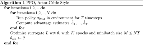
PPO is an on-policy RL algorithm that attempts to improve the Trust Region Policy Optimization (TRPO) algorithm [13] . TRPO attempts to control the policy updates through a Kullback-Leibler (KL) divergence constraint, which quantifies how much a probability distribution differs from another [13] . A major disadvantage of this approach is that it’s computationally expensive. PPO clips the objective function to prevent large updates to the policy [14] . This make PPO easier to implement and computationally faster. The clipped objective function is shown in Equation (1).

$L^{CLIP}\left(\theta \right)={\hat{\mathbb{E}}}_t\left[\text{min}\left(\frac{{\pi }_{\theta }\left(a_t\mathrm{<mo>\; |\; </mo>}{s}_t\right)}{{\pi }_{{\theta }_{\text{old}}}\left(a_t\mathrm{<mo>\; |\; </mo>}{s}_t\right)}{\hat{A}}_t\right)\mathrm{,}\text{clip}\left(\frac{{\pi }_{\theta }\left(a_t\mathrm{<mo>\; |\; </mo>}{s}_t\right)}{{\pi }_{{\theta }_{\text{old}}}\left(a_t\mathrm{<mo>\; |\; </mo>}{s}_t\right)}\mathrm{,1}-\epsilon \mathrm{,1}+\epsilon \right){\hat{A}}_t\right]$ (1)

where ${\pi }_{\theta }$ is a stochastic policy. The clipping function limits the lower and upper value of the probability ratio $\frac{{\pi }_{\theta }\left(a_t\mathrm{<mo>\; |\; </mo>}{s}_t\right)}{{\pi }_{{\theta }_{\text{old}}}\left(a_t\mathrm{<mo>\; |\; </mo>}{s}_t\right)}$ and $\epsilon$ is the hyperparameter that sets the clip range. The larger the value of $\epsilon$ , the larger the potential policy changes. ${\hat{A}}_t$ is the advantage function shown in Equation (2).

${\hat{A}}_t={\delta }_t+\left(\gamma \lambda \right){\delta }_{t+1}+\cdots +{\left(\gamma \lambda \right)}^{T-t+1}{\delta }_{T-1}$ (2)

where ${\delta }_t$ is the TD error defined in Equation (3), $\gamma$ is the discount factor, and $\lambda$ is the bias-variance trade-off factor for the generalized advantage estimator [15] . During each episode of training, the actor collects T timesteps of data. Then, the surrogate loss is computed over T timesteps and optimized with minibatch stochastic gradient descent for K epochs. Algorithm 1 summarizes the training process for PPO. As training progresses, the policy will try to exploit rewards already found over exploration.

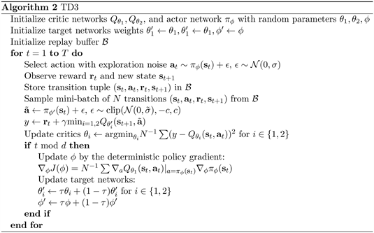
TD3 is an off-policy algorithm that significantly improves upon the deep deterministic policy gradient (DDPG) algorithm [16] . The primary downfall of DDPG is the overestimation bias of the critic network, which leads to degraded performance. TD3 implements three key features to improve performance [17] . First, TD3 proposes the use of a clipped double Q-learning algorithm to replace

the standard Q-learning found in DDPG. The second feature implemented is the use of action noise to reduce overfitting to narrow peaks in the value estimate, a problem often encountered with deterministic policies. The addition of action noise also results in target policy smoothing. For each timestep, both Q networks ( $Q_{{\theta }_1}\mathrm{,}{Q}_{{\theta }_2}$ ) are updated towards the minimum target value of actions selected by the target policy shown in Equation (3)

$y=r_t+\gamma \underset{i=1,2}{\min }{Q}_{{{\theta }^{\prime }}_i}\left(s_{t+1},{\pi }_{{\varphi }^{\prime }}\left(s_{t+1}\right)+\epsilon \right).$ (3)

where $r_t$ is the reward at time t, $\gamma$ is the discount factor and ${\pi }_{\varphi }$ is a deterministic policy, with parameters $\varphi$ , which maximizes the expected return. $\epsilon$ is the clipped Gaussian action noise added and is defined by Equation (4).

$\epsilon ~\text{clip}\left(\mathcal{N}\left(\mathrm{0,}\sigma \right)\mathrm{,}-c\mathrm{,}c\right)$ (4)

The third feature of TD3 is to delay the policy updates by a fixed number of updates to the critic. This is done to suppress the value estimate variance caused by the accumulated TD error. Parameters $\varphi$ are updated according to the deterministic policy gradient shown in Equation (5).

${\nabla }_{\varphi }J\left(\varphi \right)={\mathbb{E}}_{s_t~p_{\pi }}\left[{{\nabla }_a{Q}_{\pi }\left(s_t\mathrm{,}{a}_t\right)|}_{a_t={\pi }_{\varphi }\left(s_t\right)}{\nabla }_{\varphi }{\pi }_{\varphi }\left(s_t\right)\right]\mathrm{.}$ (5)

where $Q_{\pi }$ is the action-value function defined in Equation (5). TD3 is summarized in algorithm 2.

SAC is an off-policy actor-critic algorithm that seeks to maximize a trade-off between expected return and entropy. This encourages a high degree of exploration compared to other algorithms. The entropy augmented objective is defined by Equation (6).

${\pi }^{\mathrm{<mo>\; *\; </mo>}}=\underset{\pi }{\arg \max }{\displaystyle \underset{t}{\sum }}{\mathbb{E}}_{\left(s_t\mathrm{,}{a}_t\right)~{\rho }_{\pi }}\left[r_t+\alpha \mathcal{H}\left(\pi \left(\cdot \mathrm{<mo>\; |\; </mo>}{s}_t\right)\right)\right]\mathrm{,}$ (6)

$r_t$ is the reward at time t and $\alpha$ determines the relative importance of the entropy term, $\mathcal{H}\left(\pi \left(\cdot \mathrm{<mo>\; |\; </mo>}{s}_t\right)\right)=\log \left({\pi }_{\varphi }\left(a_t\mathrm{<mo>\; |\; </mo>}{s}_t\right)\right)$ , against the reward. ${\pi }_{\varphi }$ is a deterministic policy, with parameters $\varphi$ . SAC utilizes two soft Q-functions to mitigate positive bias in the policy improvement step. The soft Q-function parameters, $\theta$ , are trained to minimize the soft Bellman residual given in Equation (7).

$J_Q\left(\theta \right)={\mathbb{E}}_{\left(s_t\mathrm{,}{a}_t\right)~\mathcal{B}}\left[\frac{1}{2}{\left(Q_{\theta }\left(s_t\mathrm{,}{a}_t\right)-\left(r_t+\gamma {\mathbb{E}}_{s_{t+1}~p}\left[V_{\bar{\theta }}\left(s_{t+1}\right)\right]\right)\right)}^2\right]\mathrm{,}$ (7)

where $Q_{\theta }\left(s_t\mathrm{,}{a}_t\right)$ is the minimum of the two soft Q-functions and $\gamma$ is the discount factor. The value function $V_{\theta }$ is the value function implicitly parameterized through the soft Q-function parameters via Equation (8).

$V\left(s_t\right)\mathrm{<mo>\; =\; </mo>}{\mathbb{E}}_{a_t~\pi }\left[Q\left(s_t\mathrm{,}{a}_t\right)-\alpha \log \pi \left(a_t\mathrm{<mo>\; |\; </mo>}{s}_t\right)\right]$ (8)

The policy parameters are trained by minimizing the objective function in Equation (9).

$J_{\pi }\left(\varphi \right)={\mathbb{E}}_{s_t~\mathcal{B}}\left[{\mathbb{E}}_{a_t~{\pi }_{\varphi }}\left[\alpha \log \left({\pi }_{\varphi }\left(a_t|s_t\right)\right)-Q_{\theta }\left(s_t\mathrm{,}{a}_t\right)\right]\right].$ (9)

Additionally, the temperature parameter $\alpha$ can be learned with the following objective function in Equation (10).

$J\left(\alpha \right)={\mathbb{E}}_{a_t~{\pi }_t}\left[-\alpha \log {\pi }_t\left(a_t\mathrm{<mo>\; |\; </mo>}{s}_t\right)-\alpha \bar{\mathcal{H}}\right]$ (10)

The pseudo-code for SAC is listed in Algorithm 3. SAC alternates between collecting experience from the environment with the current policy and updating the actor and critic network parameters using stochastic gradients from batches randomly sampled from a replay buffer [18] .

4. Experimental Setup

In this section, the hardware and software components of the quadruped robot testbed used to evaluate the RL algorithms are discussed.

4.1. Robot

Figure 1 shows the simulated robot used in pretraining the RL algorithms. This work was discussed in our previous paper, “A Comparison of PPO, TD3, and SAC Reinforcement Learning Algorithms for Quadruped Walking Gait Generation” [19] . The robot shown in Figure 2 is the real-world counterpart to the

Figure 1. Simulated quadruped robot testbed.

Figure 2. Quadruped robot testbed used for real-world testing and training.

simulated robot. The sensors on the real robot are nearly identical to those used with the simulated robot. This was done so that models trained in simulation could be directly implemented on the real robot without any changes.

4.2. Controller

The controller hardware of the robot is a Jetson Xavier AGX development board from NVIDIA shown in Figure 2. The controller consists of an 8-core, 64-bit ARM CPU with an NVIDIA GPU containing 512 CUDA and 64 tensor cores. The controller also has 64 GB of LPDDR4x RAM for volatile memory and uses a 500 GB NVMe solid-state drive for non-volatile memory. Lastly, the controller has several I/O interfaces, including an M.2 Key E slot for dual-band WiFi, multiple USB ports, and I2C buses.

The controller software handles all policy inferences and updates, sensory data collection, and actuator control. Sequential queries of the various sensors introduce significant delay; therefore, the code to read each sensor was implemented in its own kernel process for asynchronous data collection. The data can then be accessed via shared memory.

4.3. Actuators

The testbed uses eight Dynamixel XC430-W240-T metal gear smart servo actuators in the four legs, as shown in Figure 2. The servos communicate at a baud rate of 4 Mbits per second with the Dynamixel USB communication converter (U2D2), which is interfaced with the Jetson Xavier AGX, enabling the software to control the individual servos. Each servo provides load, velocity, position, temperature, and error status to the Jetson approximately at the sampling frequency of 200 Hz. The temperature and error status signals are used only to monitor the robot’s operating conditions and pause training if normal operating conditions are violated. Additionally, each servo implements its own internal PID loop to smooth joint motions.

4.4. Position Tracking

Position tracking is implemented using the Zed mini stereo camera from Stereolabs. Real-time depth-based visual odometry and SLAM algorithms are used to compute translation and orientation with an accuracy of 0.01 meters and 0.1 degrees, respectively. The accuracy of the real-time depth-based visual odometry and SLAM algorithms depends on the scene captured by the camera. The camera provides translation in a three-dimensional Cartesian coordinate system (X, Y, Z) and provides orientation in the form of a quaternion (w, x, y, z). The camera collects and processes images at a sampling rate of 100 Hz and communicates with the Jetson Xavier AGX over the USB.

4.5. Contact Sensing

The testbed uses four force-resistive sensors located on the bottom of each robot’s feet for contact sensing. The sensors are connected to a 16-bit analog-to-digital converter (ADC) interfaced with the Jetson Xavier AGX using the I2C bus. The contact sensory data is sampled at approximately 150 Hz.

4.6. Inertial Measurement

The robot has nine inertial measurement units (IMU), with each IMU having 9 Degrees of Freedom (DOF), to collect proprioceptive information of the robot body and legs as shown in Figure 2. Each IMU contains a three-axis accelerometer, three-axis gyro, and three-axis magnetometer. One IMU is located on the center body above the camera. The remaining eight IMUs are located on the legs. One IMU is located on the upper portion of each leg, and another on the lower section of each leg. The IMUs are interfaced to the Jetson Xavier AGX using a multiplexer over the second I2C bus. The accelerometer and gyro data values from the IMUs are sampled at approximately 140 Hz. The magnetometer values are not queried or used in this research.

4.7. State and Action Spaces

Actions $a_t$ are actuator target positions mapped to values between −1 and 1. The state $s_t$ consists of the most recent readings of various sensors. Seven sensor configurations were tested with each algorithm to identify the best possible level of sensory input for each algorithm. Table 1 lists the sensors used in each configuration. The first configuration (v0) uses only the body quaternion for the state space, and the last configuration (v6) utilizes all sensor data on the robot for the state space.

4.8. Reward Function

The reward function was designed to encourage a stable forward walking gait at a target velocity ${\hat{v}}_x$ with a target orientation $\hat{q}$ . The reward function is given by the Equation (14)

$\begin{array}{c}R=r_H+w_A\ast {\displaystyle \sum }{\left(a_t\right)}^2+w_V\ast {\displaystyle \sum }{\left({\Omega }_t\right)}^2+w_{TV}\ast \left|{\hat{v}}_x-v_x\right|\\ +w_D\ast \left|v_y\right|+w_{TQ}\ast \text{sum}\left(\left|\hat{q}-q\right|\right),\end{array}$ (11)

Table 1. State space configurations.

where $r_H$ is the reward for not experiencing a catastrophic failure, such as flipping over. $w_A$ is the weight that determines the importance of penalizing actions, $a_t$ . $w_V$ is the weight that determines the importance of penalizing actuator velocities, ${\Omega }_t$ . $w_{TV}$ is the importance weight for the target velocity, and $w_D$ is the importance weight for penalizing linear velocity in the lateral direction. $w_{TQ}$ is the importance weight for deviation from the target quaternion. The final weights used are listed in Table 2.

4.9. Training

A simulated environment is set up to recreate the agent environment described previously. Every 50 ms in simulation time, the agent reads the current state of the robot, which is described by the robot’s sensors. The sensors that are used depend on which configuration is being tested. The agent then uses the state space to generate target motor positions. The updated motor positions are sent to the robot. After 50 ms, the robot’s state is read again, and a reward is given based on the reward function described in section 1. This process is repeated for one thousand iterations. The simulation is reset Upon completing an episode of a thousand steps. TD3 and SAC algorithms update following each episode’s end, while PPO updates at fixed intervals. Each algorithm is trained on each sensor configuration for three million steps. This is repeated five times for each algorithm configuration combination.

A second group of policies was trained under identical circumstances except with domain randomization to evaluate if an algorithm is suitable for transfer learning to a real robot. The group using dynamics randomization experienced random variations in the robot’s mass, inertia, and friction coefficients, as well as actuator stiffness, friction loss, damping, and reflected inertia variations.

4.10. Models and Hyper Parameters

To compare the optimal performance of each algorithm, the Stable-Baselines3 (SB3) implementation was used for all three algorithms. SB3 is a set of reliable implementations of reinforcement learning algorithms in PyTorch [20] . Several combinations of hyperparameters were tested for each algorithm. However, the default SB3 values were found to be the best. Table 3 summarizes each algorithm’s ANN architectures and hyperparameters.

4.11. Performance Metrics

The performance of trained policies was evaluated through several quantitative metrics of a walking gait. These metrics include average forward velocity (m/s), average forward velocity variance, average lateral velocity (m/s), average lateral

Table 2. Reward function parameters.

Table 3. Hyperparameters for each RL algorithm.

velocity variance, and quaternion root mean square deviation (RMSD). The most important metric is the forward velocity. Ideally, an agent should achieve an average forward velocity of 0.5 m/s, a lateral velocity of 0.0 m/s, no forward or lateral velocity variance, and no deviation in the quaternion. The algorithm considered the “best” would be the one that achieves a forward velocity closest to the target velocity of 0.5 m/s.

5. Results

This section presents the results of transferred agents’ performance before and after real-world training.

5.1. Training without Domain Randomization

For PPO, only four configurations, v1, v2, v3, and v4, were tested on the robot since configurations v0, v5, and v6 did not generate a walking gait with a forward velocity close to 0.5 m/s in the simulation. Similarly, for TD3, only configurations v2, v3, and v4 were transferred to the real robot for retraining. Finally, using SAC, five configurations, v2, v3, v4, v5, and v6, were selected to be retrained on the real robot. The analysis of training results in simulation was presented in our previous work [1] .

Figures 3-5 show the average reward during the fifty thousand step retraining process. It can be seen that PPO has a much higher initial reward than both TD3 and SAC. This suggests that PPO is better for transfer learning than SAC and

Figure 3. Learning curves for on-robot retraining using PPO without domain randomization pretraining.

Figure 4. Learning curves for on-robot retraining using TD3 without domain randomization pretraining.

TD3. It is worth noting that PPO has a smaller network size than TD3 and SAC. A smaller network can prevent overfitting, leading to better transfer learning. However, by the end of fifty thousand training steps, the average reward for SAC and TD3 is on par with PPO. Additionally, from the SAC learning curve, it can be seen that the average reward for configurations v5 and v6 falls as training

Figure 5. Learning curves for on-robot retraining using SAC without domain randomization pretraining.

Table 4. Gait analysis of PPO agents pretrained without domain randomization before and after real-time retraining.

progresses. This would indicate that adding the IMU data is detrimental to learning to walk in the real world. Furthermore, the retrained PPO agents show little improvement in average reward over the retraining period.

Tables 4-6 show the performance of each algorithm-configuration combination before and after retraining on the physical robot. As expected, the performance of all agents before retraining is very poor due to the reality gap. Despite having a significantly higher starting average reward, the performance of the PPO agents is not quantitatively better than TD3 or SAC on the tests conducted before retraining. Additionally, none of the agents could generate a stable walking

Table 5.Gait analysis of TD3 agents pretrained without domain randomization before and after real-time retraining.

Table 6. Gait analysis of SAC agents pretrained without domain randomization before and after real-time retraining.

gait after retraining on the robot. In most cases, the robot only learns to maintain its forward orientation and minimize erratic movements of the legs at the expense of forward movement. This is corroborated by the fact that the average forward velocity and quaternion RMSD are lower for most trials after retraining. Ultimately, no agent demonstrated significant improvements in forward velocity from retraining.

5.2. Training with Domain Randomization

The experimental results using agents pretrained with domain randomization are similar to previous results. Figures 6-8 show the learning curves for each algorithm-configuration combination using domain randomization pretraining. Similar to the simulated results, the average rewards are slightly lower than those without domain randomization. This is unexpected since domain randomization

Figure 6. Learning curves for on-robot retraining using PPO with domain randomization pretraining.

Figure 7. Learning curves for on-robot retraining using TD3 with domain randomization pretraining.

aims to help the agent generalize for better transfer learning. However, the performance of configurations v5 and v6 for SAC shows significant improvement over the agents trained without domain randomization. Unlike the agents pretrained without domain randomization, the average return does drop as training progresses. Also, surprisingly configuration v6 achieved a higher average reward than configuration v5. A similar trend was seen in the simulation.

From Tables 7-9, it can be seen that no agent generated a stable walking gait at the desired forward velocity even when pretrained with domain randomization. The walking performance for agents using TD3 and SAC is on par with those pretrained without domain randomization. However, retrained PPO agents consistently show a significantly higher forward velocity and a lower quaternion RMSD. Configuration v2 achieved the highest average forward velocity of 0.11786 m/s after being retrained on the physical robot. Despite having the highest forward velocity, this agent had the lowest average return by the end of

Figure 8. Learning curves for on-robot retraining using SAC with domain randomization pretraining.

Table 7. Gait analysis of PPO agents pretrained with domain randomization before and after real-time retraining.

Table 8. Gait analysis of TD3 agents pretrained with domain randomization before and after real-time retraining.

Table 9. Gait analysis of SAC agents pretrained with domain randomization before and after real-time retraining.

the fifty thousand training steps. However, given more training time, the agent may be able to achieve the desired forward velocity.

5.3. Results Summary

The results show that no policy trained in simulation, regardless of the algorithm or use of domain randomization, successfully transferred to the physical robot, indicating no policy trained in simulation could be used to make the physical robot walk. This shows that the simulated world differs from the real world significantly to be used to pretrain policies. Only a single PPO policy, pre-trained with domain randomization and then retrained on the physical robot, could generate a walking gait with any significant forward velocity (greater than 0.1 m/s). The policy used configuration v2, which only includes the body quaternion, actuator position, and actuator velocity. Regardless, all PPO policies pretrained with domain randomization show significant improvement in the walking gait metrics after being retrained on the physical robot. This indicated that using PPO with domain randomization is the best way to overcome the reality gap compared to TD3 and SAC. While the real-time training proved unsuccessful for the TD3 and SAC algorithms, it can not be conclusively stated that these algorithms are unsuitable for real-time learning. However, it is interesting that TD3 and SAC are off-policy algorithms and are generally considered faster learners. However, faster learning may lead to overfitting to the simulated domain. Alternatively, PPO may generalize better due to a smaller network size. This is supported by the real-time learning curves of the PPO agents, which all start with much higher rewards than the TD3 or SAC agents.

6. Conclusions and Future Work

This research has demonstrated transfer learning augmented by real-time reinforcement learning for gait generation on a quadruped robot. The effect of domain randomization before and after real-time training has been shown. From the experimental data, it appears that the PPO pretrained with domain randomization greatly improves the ability to transfer a simulated agent to the real world. Additionally, once retrained in real-time, the agents improve further. This shows that life-long learning tasks could be viable strategies for robotic applications.

In our future work, we propose to study the use of a different simulated environment focused on digital twins reflective of the real world, like Nvidia Omniverse. Also, a more robust robot like Boston Dynamic’s Spot or Unitree’s Go1 could be a more suitable testbed. Training the robots for a longer time may give some of the agents time to develop a stable walking gait. Compared to the three million training steps of the simulated environment, fifty thousand training steps on the robot is not a lot of training time. Training for an additional fifty thousand steps in the real world could lead to further improvements but still be accomplished within a single day. Furthermore, tuning of the reward function weights may be required for real-world training to prioritize forward movement. However, tuning reward weights for real-world training would be extremely time-intensive.

Conflicts of Interest

The authors declare no conflicts of interest regarding the publication of this paper.

References

[1]	Mock, J.W. and Muknahallipatna, S.S. (2023) A Comparison of PPO, TD3 and SAC Reinforcement Algorithms for Quadruped Walking Gait Generation. Journal of Intelligent Learning Systems and Applications, 15, 36-56. https://doi.org/10.4236/jilsa.2023.151003
[2]	Salvato, E., Fenu, G., Medvet, E. and Pellegrino, F.A. (2021) Crossing the Reality Gap: A Survey on Sim-to-Real Transferability of Robot Controllers in Reinforcement Learning. IEEE Access, 9, 153171-153187. https://doi.org/10.1109/ACCESS.2021.3126658
[3]	Zhao, W., Queralta, J.P. and Westerlund, T. (2020) Sim-to-Real Transfer in Deep Reinforcement Learning for Robotics: A Survey. 2020 IEEE Symposium Series on Computational Intelligence (SSCI), Canberra, 1-4 December 2020, 737-744. https://arxiv.org/abs/2009.13303 https://doi.org/10.1109/SSCI47803.2020.9308468
[4]	Xie, Z., Clary, P., Dao, J., Morais, P., Hurst, J. and van de Panne, M. (2020) Learning Locomotion Skills for Cassie: Iterative Design and Sim-to-Real. Proceedings of the Conference on Robot Learning, Vol. 100, 317-329. https://proceedings.mlr.press/v100/xie20a.html
[5]	Hwangbo, J., Lee, J., Dosovitskiy, A., Bellicoso, D., Tsounis, V., Koltun, V. and Hutter, M. (2019) Learning Agile and Dynamic Motor Skills for Legged Robots. Science Robotics, 4, eaau5872. http://arxiv.org/abs/1901.08652 https://doi.org/10.1126/scirobotics.aau5872
[6]	Tan, J., Zhang, T., Coumans, E., Iscen, A., Bai, Y., Hafner, D., Bohez, S. and Vanhoucke, V. (2018) Sim-to-Real: Learning Agile Locomotion for Quadruped Robots. http://arxiv.org/abs/1804.10332
[7]	Muratore, F., Gienger, M. and Peters, J. (2019) Assessing Transferability from Simulation to Reality for Reinforcement Learning. IEEE Transactions on Pattern Analysis and Machine Intelligence, 43, 1172-1183. http://arxiv.org/abs/1907.04685
[8]	Tobin, J., Fong, R., Ray, A., Schneider, J., Zaremba, W. and Abbeel, P. (2017) Domain Randomization for Transferring Deep Neural Networks from Simulation to the Real World. 2017 IEEE/RSJ International Conference on Intelligent Robots and Systems (IROS), Vancouver, 24-28 September 2017, 23-30. http://arxiv.org/abs/1703.06907 https://doi.org/10.1109/IROS.2017.8202133
[9]	Pinto, L., Andrychowicz, M., Welinder, P., Zaremba, W. and Abbeel, P. (2017) Asymmetric Actor Critic for Image-Based Robot Learning. http://arxiv.org/abs/1710.06542
[10]	Rudin, N., Hoeller, D., Reist, P. and Hutter, M. (2021) Learning to Walk in Minutes Using Massively Parallel Deep Reinforcement Learning. https://arxiv.org/abs/2109.11978
[11]	Mahmood, A.R., Korenkevych, D., Komer, B.J. and Bergstra, J. (2018) Setting up a Reinforcement Learning Task with a Real-World Robot. 2018 IEEE/RSJ International Conference on Intelligent Robots and Systems (IROS), Madrid, 1-5 October 2018, 4635-4640. http://arxiv.org/abs/1803.07067
[12]	Haarnoja, T., Ha, S., Zhou, A., Tan, J., Tucker, G. and Levine, S. (2019) Learning to Walk via Deep Reinforcement Learning. https://doi.org/10.15607/RSS.2019.XV.011
[13]	Schulman, J., Levine, S., Moritz, P., Jordan, M.I. and Abbeel, P. (2015) Trust Region Policy Optimization. Proceedings of the 32nd International Conference on Machine Learning, Vol. 37, 1889-1897. http://arxiv.org/abs/1502.05477
[14]	Schulman, J., Wolski, F., Dhariwal, P., Radford, A. and Klimov, O. (2017) Proximal Policy Optimization Algorithms. http://arxiv.org/abs/1707.06347
[15]	Schulman, J., Moritz, P., Levine, S., Jordan, M.I. and Abbeel, P. (2016) High-Dimensional Continuous Control Using Generalized Advantage Estimation. 4th International Conference on Learning Representations, ICLR 2016, San Juan, 2-4 May 2016. http://arxiv.org/abs/1506.02438
[16]	Lillicrap, T.P., Hunt, J.J., Pritzel, A., Heess, N., Erez, T., Tassa, Y., Silver, D. and Wierstra, D. (2016) Continuous Control with Deep Reinforcement Learning. 4th International Conference on Learning Representations, ICLR 2016, San Juan, 2-4 May 2016. http://arxiv.org/abs/1509.02971
[17]	Fujimoto, S., van Hoof, H. and Meger, D. (2018) Addressing Function Approximation Error in Actor-Critic Methods. http://arxiv.org/abs/1802.09477
[18]	Haarnoja, T., Zhou, A., Abbeel, P. and Levine, S. (2018) Soft Actor-Critic: Off-Policy Maximum Entropy Deep Reinforcement Learning with a Stochastic Actor. http://arxiv.org/abs/1801.01290
[19]	Mock, J. and Muknahallipatna, S. (2023) A Comparison of PPO, TD3 and SAC Reinforcement Algorithms for Quadruped Walking Gait Generation. Journal of Intelligent Learning Systems and Applications, 15, 36-56. https://doi.org/10.4236/jilsa.2023.151003
[20]	Raffin, A., Hill, A., Gleave, A., Kanervisto, A., Ernestus, M. and Dormann, N. (2021) Stable-Baselines3: Reliable Reinforcement Learning Implementations. Journal of Machine Learning Research, 22, 1-8. http://jmlr.org/papers/v22/20-1364.html