Flexible Reduced Logarithmic-Inverse Lomax Distribution with Application for Bladder Cancer

Mohamed M. Buzaridah, Dina A. Ramadan, Beih S. El-Desouky

Department of Mathematics, Faculty of Science, Mansoura University, Mansoura, Egypt.

DOI: 10.4236/ojmsi.2021.94023                

Abstract

In this paper, a new method for adding parameters to a well-established distribution to obtain more flexible new families of distributions is applied to the inverse Lomax distribution (IFD). This method is known by the flexible reduced logarithmic-X family of distribution (FRL-X). The proposed distribution can be called a flexible reduced logarithmic-inverse Lomax distribution (FRL-IL). The statistical and reliability properties of the proposed models are studied including moments, order statistics, moment generating function, and quantile function. The estimation of the model parameters by maximum likelihood and the observed information matrix are also discussed. In order to assess the potential of the newly created distribution. The extended model is applied to real data and the results are given and compared to other models.

Keywords

Lomax Distribution, Inverse Lomax Distribution, Hazard Rate Function, Maximum Likelihood Estimators, Skewness and Kurtosis, Moment Generating Function

1. Introduction

Survival analysis is the branch of statistics that uses as a random variable the study of time. Before the event of the analysis occurs, such as mortality in species and breakdown of mechanical structures or facilities, this subject is referred to in engineering as reliability theory or reliability analysis, duration analysis or duration modeling in economics, and analysis of event history in sociology. Accordingly, A variety of distributions have been suggested to serve as templates for wide-ranging implementations of real-life data. Lomax [1] suggested a model for lifetime analysis, and actuarial science, known as Lomax or Pareto Type II, is a special case of the second type of generalized beta distribution. Wide applications such as the study of business failure lifetime data, income and wealth disparity, urban size, actuarial science, medical and biological sciences, engineering, lifetime and reliability modeling have been described in this distribution. Also, it has been shown its utilities for modeling and analyzes lifetime data in medical and biological sciences, engineering, etc. So, it has gained the greatest attention from theoreticians and statisticians because of its numerous uses. Hassan and Al-Ghamdi [2] developed step stress accelerated life testing for Lomax distribution. Although Corbelini et al. [3] used it to model firm size and queuing problems. Some authors, such as Bryson [4] used this distribution as an alternative to the exponential distribution when the data is heavy-tailed and has been proposed.

The Lomax distribution with two parameters, $\alpha$ and $\beta$ has a random variable X if it has a cumulative distribution function (CDF) given by

$F\left(x\right)=1-{\left[1+\frac{x}{\beta }\right]}^{-\alpha },x>0,$ (1)

where, $\beta >0$ and $\alpha >0$ are the shape and scale parameters respectively. The probability density function (PDF) is

$f\left(x\right)=\frac{\alpha }{\beta }{\left[1+\frac{x}{\beta }\right]}^{-\left(\alpha +1\right)},x>0,\beta ,\alpha >0.$ (2)

The inverse Lomax distribution is one of the significant lifetime models, and it is used in economic sciences, geography, econometrics and clinical fields; the inverse Lomax distribution was used by Kleiber [5] to obtain the Lorenz ranking relationship between the ranked stats. This distribution was used for reliability estimation based on censored Type II observations by Yadav et al. [6]. Rahman et al. [7] discussed the estimated and predicted values using Bayesian approach under various loss functions. The reliability estimators of the inverse Lomax distribution under Type II censoring were tested by Singh and Singh [8]. The Bayesian estimate of the two-component inverse Lomax distribution mixture based on the Type-I censoring scheme was discussed by Reyad and Othman [9].

The cumulative distribution function (CDF) of inverse Lomax distribution ILD with parameters $\alpha$ and $\beta$ are given by

$F\left(x\right)={\left[1+\frac{\beta }{x}\right]}^{-\alpha },x>0,\beta ,\alpha >0,$ (3)

and the corresponding probability density function (PDF) is

$f\left(x\right)=\frac{\text{d}}{\text{d}x}F\left(x\right)=\frac{\alpha \beta }{x^2}{\left[1+\frac{\beta }{x}\right]}^{-\left(\alpha +1\right)},x>0,\beta ,\alpha >0.$ (4)

Recently, Shanker and Shukla [10] introduced the generalization of generalized Gamma distribution. The Gamma-Weibull G family of distributions was introduced by Oluyede et al. [11] with applications to real-life data. Maiti and Pramanik [12] proposed a new class of distributions called odds XGamma-G family of distributions for modeling lifetime data. Korkmaz et al. [13] proposed a new class of lifetime distributions called the generalized odd Weibull generated family. Aslam et al. [14] proposed a new family of distributions, namely a modified T-X family of distributions with three most attractive features: flexibility, efficiency and parsimony. The applications of generalized distributions have been discussed with many researchers, and the reader can refer to Gallardo et al. [15], Al-Saiary et al. [16], Bantan et al. [17], Al-Babtain et al. [18], and Al-Babtain et al. [19].

Yinglin Liu et al. [20] proposed a new family of distributions with medical data sets. The family that is proposed may be named as a flexible reduced logarithmic-X family. Reparameterization of the exponentiated Kumaraswamy G-logarithmic family and the alpha logarithmic distribution family can be used to obtain the proposed family. In modeling complex types of data, the proposed distribution would be quite flexible. Thus, the reason for proposing the FRL-X family is to decrease the number of parameters and to relax the boundary conditions of the parametric values so that the hazard rate function is more flexible than the classical monotone behavior. Also, this provides us more knowledge about the behavior of the hazard rate function in the tail end to improve the description that calls for complexity by adding the parameters in the class of distributions. A random variable X is said to have the FRL-X distribution if it (CDF) is given by

$G\left(x;\lambda ,\xi \right)=1-\frac{\log \left[1+\lambda -\lambda F\left(x;\xi \right)\right]}{\log \left[1+\lambda \right]},\lambda >0,x\in ℝ,$ (5)

where depending on the parameter $\xi$, $F\left(x\mathrm{<mo>\; ;\; </mo>}\xi \right)$ is CDF of the baseline random variable and $\lambda$ is an additional parameter. The term in Equation (5) is also true for $\lambda =1$. The probability density function (PDF) corresponding to Equation (5) is given by

$g\left(x\mathrm{<mo>\; ;\; </mo>}\lambda \mathrm{,}\xi \right)=\frac{\text{d}}{\text{d}x}F\left(x\right)=\frac{\lambda f\left(x\mathrm{<mo>\; ;\; </mo>}\xi \right)}{\left[1+\lambda -\lambda F\left(x\mathrm{<mo>\; ;\; </mo>}\xi \right)\right]\log \left[1+\lambda \right]}\mathrm{,}x\in ℝ\mathrm{.}$ (6)

The reliability or survival function $S\left(x\right)$ and failure rate or hazard rate function $S\left(x\right)$, of the flexible reduced logarithmic-X (FRL-X) distribution, is given by

$S\left(x;\lambda ,\xi \right)=P\left(X>x\right)=1-G\left(x;\lambda ,\xi \right)=\frac{\log \left[1+\lambda -\lambda F\left(x;\xi \right)\right]}{\log \left(1+\lambda \right)},x\in ℝ,$ (7)

and

$h\left(x;\lambda ,\xi \right)=\frac{g\left(x;\lambda ,\xi \right)}{S\left(x;\lambda ,\xi \right)}=\frac{\lambda f\left(x;\xi \right)}{\left[1+\lambda -\lambda F\left(x;\xi \right)\right]\log \left[1+\lambda -\lambda F\left(x;\xi \right)\right]},x\in ℝ.$ (8)

In addition to the above, the main reasons for using the FRL-X family in practice are:

1) The possibility of adding additional parameters in a simple way to modify the existing distributions.

2) To improve the features and flexibility of existing distributions.

3) To show the extended version of the baseline distribution having closed forms for cumulative distribution function, hazard rate function, and survival function.

4) To provide better measurements than the corresponding modified models.

5) To add new distributions having nonmonotonic shaped hazard rate functions.

6) To insert the best fit to unimodal medical care data sets.

This paper is structured as follows: The FRL-X family, called the flexible logarithmic-inverse Lomax (FRL-IL) distribution, was introduced in Section 2. The structural characteristics of the distribution of FRL-IL include the behavior of the function of probability density, the reliability or survival function, the function of the hazard rate, the function of the reversed hazard rate, the residual (reversed) life. The moments and the moments generating function, quantile function, and skewness and kurtosis are given in Section 3. Section 4 provides order statistics and extreme values. The maximum likelihood estimation of the unknown parameters is discussed in Section 5. Finally, in Section 6, a real data life application has shown up the potential of FRL-IL distribution relative to other distributions.

2. The Flexible Reduced Logarithmic-Inverse Lomax (FRL-IL) Distribution

It is said that the random variable X has flexible reduced distribution logarithmic-inverse Lomax (FRL-IL) denoted by FRL-IL $\left(\alpha \mathrm{,}\beta \mathrm{,}\lambda \right)$. Let $F\left(x\mathrm{<mo>\; ;\; </mo>}\xi \right)$ and $f\left(x\mathrm{<mo>\; ;\; </mo>}\xi \right)$ be cumulative distribution function (CDF) and probability density function (PDF) of the two-parameter inverse Lomax distribution. Using $F\left(x\right)$ and $f\left(x\right)$ from Equations (3) and (4), respectively, in Equations (5) and (6) to obtain, the (CDF) of the FRL-IL distribution is given by

$F\left(x;\alpha ,\beta ,\lambda \right)=1-\frac{\log \left[1+\lambda -\lambda {\left(1+\frac{\beta }{x}\right)}^{-\alpha }\right]}{\log \left[1+\lambda \right]},x>0,\alpha ,\beta ,\lambda >0.$ (9)

The probability density function (PDF) corresponding to Equation (6) is given by

$f\left(x;\alpha ,\beta ,\lambda \right)=\frac{\frac{\alpha \beta \lambda }{x^2}{\left[1+\frac{\beta }{x}\right]}^{-\left(\alpha +1\right)}}{\left[1+\lambda -\lambda {\left(1+\frac{\beta }{x}\right)}^{-\alpha }\right]\log \left[1+\lambda \right]},x>0,\alpha ,\beta ,\lambda >0,$ (10)

The survival function or reliability $S\left(x\right)$, failure rate or hazard rate function $h\left(x\right)$, reversed-hazard rate function $r\left(x\right)$, and cumulative hazard rate function $H\left(x\right)$ of the flexible reduced logarithmic-inverse Lomax (FRL-IL) distribution are given by

$S\left(x;\alpha ,\beta ,\lambda \right)=\frac{\log \left[1+\lambda -\lambda {\left(1+\frac{\beta }{x}\right)}^{-\alpha }\right]}{\log \left(1+\lambda \right)},x>0,$ (11)

$\begin{array}{l}h\left(x;\alpha ,\beta ,\lambda \right)\\ =\frac{\frac{\alpha \beta \lambda }{x^2}{\left(1+\frac{\beta }{x}\right)}^{-\left(\alpha +1\right)}}{\left[1+\lambda -\lambda {\left(1+\frac{\beta }{x}\right)}^{-\alpha }\right]\log \left[1+\lambda -\lambda {\left(1+\frac{\beta }{x}\right)}^{-\alpha }\right]},x>0,\end{array}$ (12)

$\begin{array}{l}r\left(x;\alpha ,\beta ,\lambda \right)\\ =\frac{\alpha \beta \lambda x^{-2}{\left(1+\frac{\beta }{x}\right)}^{-\left(\alpha +1\right)}}{\left[\log \left(1+\lambda \right)-\log \left\{1+\lambda -\lambda {\left(1+\frac{\beta }{x}\right)}^{-\alpha }\right\}\right]\left[1+\lambda -\lambda {\left(1+\frac{\beta }{x}\right)}^{-\alpha }\right]},x>0,\end{array}$ (13)

and

$\begin{array}{c}H\left(x;\alpha ,\beta ,\lambda \right)={\displaystyle {\int }_0^x}h\left(u\right)\text{d}u=-\log S\left(x;\alpha ,\beta ,\lambda \right)\\ =-\log \left(\frac{\log \left[1+\lambda -\lambda {\left(1+\frac{\beta }{x}\right)}^{-\alpha }\right]}{\log \left(1+\lambda \right)}\right),\end{array}$ (14)

respectively, $x>0$ and $\alpha ,\beta ,\lambda >0$.

Figures 1-6 show the PDF, CDF, survival function $S\left(x\right)$, hazard rate function $h\left(x\right)$, reversed hazard rate function $r\left(x\right)$ and cumulative hazard rate function $H\left(x\right)$ of the FRL-IL $\left(\alpha \mathrm{,}\beta \mathrm{,}\lambda \right)$ distribution for some parameter values.

Figure 1. The pdf of the FRL-IL for different values of parameters.

Figure 2. The CDF of the FRL-IL for different values of parameters.

Figure 3. The S(x) of the FRL-IL for different values of parameters.

Figure 4. The h(x) of the FRL-IL for different values of parameters.

Figure 5. The r(x) of the FRL-IL for different values of parameters.

Figure 6. The H(x) of the FRL-IL for different values of parameters.

3. Some Statistical Properties

In this section, we give some statistical properties of FRL-IL distribution.

3.1. Quantile Function and Median

The quantile function has a number of important applications, for example, it can be used to obtain the median, skewness, kurtosis and can be also used to generate random variables. Suppose X a random variable from the FRL-IL distribution with CDF from Equation (10), the quantile function of X, is given by

$x=Q\left(u\right)=F^{-1}\left(u\right)=F^{-1}\left(\frac{1+\lambda -{\text{e}}^{\log \left(1+\lambda \right)\left(1-u\right)}}{\lambda }\right),$ (15)

where $u\sim uniform\left(\mathrm{0,1}\right)$ from the FRL-IL distribution, random numbers can easily be generated using

$x=\frac{\beta {\lambda }^{-\frac{1}{\alpha }}}{{\left(1+\lambda -{\text{e}}^{\left(1-u\right)\log \left(1+\lambda \right)}\right)}^{-\frac{1}{\alpha }}-{\lambda }^{-\frac{1}{\alpha }}}\mathrm{.}$ (16)

It is possible to derive the median of the FRL-IL distribution by setting $u=0.5$ in Equation (16) to be

$median=\frac{\beta {\lambda }^{-\frac{1}{\alpha }}}{{\left(1+\lambda -{\text{e}}^{0.5\log \left(1+\lambda \right)}\right)}^{-\frac{1}{\alpha }}-{\lambda }^{-\frac{1}{\alpha }}}\mathrm{.}$ (17)

3.2. Mode of the FRL-IL Distribution

The mode of the flexible reduced logarithmic-inverse Lomax (FRL-IL) distribution is derived by differentiating the probability density function in Equation (10) with respect to random variable $x>0$ and equal it to zero.

So, then the mode is the solution of the following equation

$\begin{array}{l}\frac{\left[\left(1+\lambda -\lambda {\left(1+\frac{\beta }{x}\right)}^{-\alpha }\right)\log \left(1+\lambda \right)\right]\left[\left(\frac{\alpha \beta \lambda }{x^2}\right)\left(\frac{\beta }{x^2}\left(\alpha +1\right){\left(1+\frac{\beta }{x}\right)}^{-\left(\alpha +2\right)}\right)-\left({\left(1+\frac{\beta }{x}\right)}^{-\left(\alpha +1\right)}\right)\left(\frac{2\alpha \beta \lambda }{x^3}\right)\right]}{{\left(\left[1+\lambda -\lambda {\left(1+\frac{\beta }{x}\right)}^{-\alpha }\right]\log \left[1+\lambda \right]\right)}^2}\\ -\frac{\left[\left(\frac{\alpha \beta \lambda }{x^2}\right)\left({\left(1+\frac{\beta }{x}\right)}^{-\left(\alpha +1\right)}\right)\right]\left[\left(\log \left(1+\lambda \right)\left(\frac{\alpha \beta \lambda }{x^2}{\left(1+\frac{\beta }{x}\right)}^{-\left(\alpha +1\right)}\right)\right)\right]}{{\left(\left[1+\lambda -\lambda {\left(1+\frac{\beta }{x}\right)}^{-\alpha }\right]\log \left[1+\lambda \right]\right)}^2}=0.\end{array}$ (18)

3.3. Skewness and Kurtosis

One of the most common methods to measure the skewness and kurtosis of a distribution is to consider measures defined with moments. However, moments cannot always be found. This applies true for heavy-tailed distributions such as the Lomax or inverse Lomax distribution. For this reason, the use of the quantile function offers some alternatives. The shortcomings of the conventional measure of kurtosis are well known. Kenney and Keeping [21] provides the skewness of Bowely on the basis of quantities as

$S_k=\frac{q_{\left(0.75\right)}-2q_{\left(0.5\right)}+q_{\left(0.25\right)}}{q_{\left(0.75\right)}-q_{\left(0.25\right)}}.$ (19)

Moors [22] gave the Moors quantile based Kurtosis as

$K_u=\frac{q_{\left(0.875\right)}-q_{\left(0.625\right)}-q_{\left(0.375\right)}-q_{\left(0.125\right)}}{q_{\left(0.75\right)}-q_{\left(0.25\right)}}\mathrm{,}$ (20)

with the $q_{\left(\mathrm{.}\right)}$ representing quantile function.

The sign of S is informative on the direction of the skewness of the distribution $S>0$ for right-skewed, $S=0$ for symmetric, and $S<0$ for left-skewed. The value of K measures the tail-heaviness of the distribution; in general, the bigger is the value of K is the heavier is the tail of the distribution.

3.4. Moments

Given the importance of the rth moments in any statistical analysis in applications, as they can be used to study the most important features and characteristics of the distribution (such as slope, dispersion, skew and kurtosis), in this subsection we will discuss how to find the rth moments of the FRL-IL distribution, which are derived is be given by

$\begin{array}{c}{{\mu }^{\prime }}_r=E\left(x^r\right)\\ ={\displaystyle {\int }_0^{\infty }}{x}^{r}f\left(x;\alpha ,\beta ,\lambda \right)\text{d}x.\end{array}$ (21)

By replacing Equation (10) with Equation (21), we get

${{\mu }^{\prime }}_r={\displaystyle {\int }_0^{\infty }}{x}^r\frac{\frac{\alpha \beta \lambda }{x^2}{\left(1+\frac{\beta }{x}\right)}^{-\left(\alpha +1\right)}}{\left(1+\lambda -\lambda {\left(1+\frac{\beta }{x}\right)}^{-\alpha }\right)\log \left(1+\lambda \right)}\text{d}x,$

where $\left(1+\lambda -\lambda {\left(1+\frac{\beta }{x}\right)}^{-\alpha }\right)=\left(1+\lambda \right)\left(1-\frac{\lambda }{\lambda +1}{\left(1+\frac{\beta }{x}\right)}^{-\alpha }\right)$

${{\mu }^{\prime }}_r={\displaystyle {\int }_0^{\infty }}{x}^r\frac{\alpha \beta \lambda x^{-2}{\left(1+\frac{\beta }{x}\right)}^{-\left(\alpha +1\right)}}{\left(1+\lambda \right)\log \left(1+\lambda \right)}\left(1+\lambda \right){\left(1-\frac{\lambda }{\lambda +1}{\left(1+\frac{\beta }{x}\right)}^{-\alpha }\right)}^{-1}\text{d}x,$

where ${\left(1-\frac{\lambda }{\lambda +1}{\left(1+\frac{\beta }{x}\right)}^{-\alpha }\right)}^{-1}=\underset{i=1}{\stackrel{\infty }{{\displaystyle \sum }}}{\left(-1\right)}^i\left(\begin{array}{c}-1\\ i\end{array}\right){\left(\frac{\lambda }{\lambda +1}\right)}^{i+1}{\left(1+\frac{\beta }{x}\right)}^{-\lambda i}$, by using binomial expansion, where binomial expansion is giving by equation

${\left(a+b\right)}^n=\underset{k=0}{\stackrel{n}{{\displaystyle \sum }}}\left(\begin{array}{c}n\\ k\end{array}\right)a^k{b}^{n-k}$

${{\mu }^{\prime }}_r=\underset{i=1}{\stackrel{\infty }{{\displaystyle \sum }}}{\left(-1\right)}^i\left(\begin{array}{c}-1\\ i\end{array}\right){\left(\frac{\lambda }{\lambda +1}\right)}^{i+1}\frac{\alpha \beta }{\log \left(1+\lambda \right)}{\displaystyle {\int }_0^{\infty }}{x}^{r-2}{\left(1+\frac{\beta }{x}\right)}^{-\left(i+1\right)\alpha -1}\text{d}x.$

Let $z=\frac{\beta }{x}$ and $x=\beta z^{-1}$ then $\text{d}x=-\beta z^{-2}\text{d}z$

$\begin{array}{c}{{\mu }^{\prime }}_r=\underset{i=1}{\stackrel{\infty }{{\displaystyle \sum }}}{\left(-1\right)}^i\left(\begin{array}{c}-1\\ i\end{array}\right){\left(\frac{\lambda }{\lambda +1}\right)}^{i+1}\frac{\alpha \beta }{\log \left(1+\lambda \right)}{\displaystyle {\int }_0^{\infty }}\left(-{\beta }^{r-1}\right)z^r{\left(1+z\right)}^{-\left(i+1\right)\alpha -1}\text{d}z\\ =\underset{i=1}{\stackrel{\infty }{{\displaystyle \sum }}}{\left(-1\right)}^{i+1}\left(\begin{array}{c}-1\\ i\end{array}\right){\left(\frac{\lambda }{\lambda +1}\right)}^{i+1}\frac{\alpha {\beta }^r}{\log \left(1+\lambda \right)}B\left(-r+1,\left(i+1\right)\alpha +r\right).\end{array}$ (22)

3.5. The Moment Generating Function

The moment generating function (MGF) of the flexible reduced logarithmic-inverse Lomax (FRL-IL) distribution is follows

$M_X\left(t\right)={\displaystyle {\int }_0^{\infty }}{\text{e}}^{tx}f\left(x\mathrm{<mo>\; ;\; </mo>}\alpha \mathrm{,}\beta \mathrm{,}\lambda \right)\text{d}x\mathrm{.}$ (23)

Hence, expanding $M_X\left(t\right)$ using Taylor series yields

$M_X\left(t\right)=\underset{r=1}{\stackrel{\infty }{{\displaystyle \sum }}}\frac{t^r}{r!}{\displaystyle {\int }_0^{\infty }}{x}^{r}f\left(x;\alpha ,\beta ,\lambda \right)\text{d}x$ (24)

$=\underset{r,i=1}{\stackrel{\infty }{{\displaystyle \sum }}}{\left(-1\right)}^{i+1}\left(\begin{array}{c}-1\\ i\end{array}\right){\left(\frac{\lambda }{\lambda +1}\right)}^{i+1}\frac{\alpha {\left(\beta t\right)}^r}{r!\log \left(1+\lambda \right)}B\left(-r+1,\left(i+1\right)\alpha +r\right).$ (25)

4. The Order Statistics

Assuming that $X_{\left(1\right)}\mathrm{,}{X}_{\left(2\right)}\mathrm{,}\cdots \mathrm{,}{X}_{\left(n\right)}$ are the order statistics of a random sample follows a continuous distribution with cumulative distribution function (CDF) $F\left(x\right)$ and probability density function (PDF) $f\left(x\right)$, then the PDF of $X_{\left(k\right)}$ is given by

$f_{\left(k:n\right)}\left(x\right)=\frac{n!}{\left(k-1\right)!\left(n-k\right)!}f\left(x\right){\left[F\left(x\right)\right]}^{k-1}{\left[1-F\left(x\right)\right]}^{n-k},k=1,2,\cdots ,n.$ (26)

Let X be a random variable of FRL-IL distribution, then the density function of the k-th order statistics of the FRL-IL distribution is

$\begin{array}{c}{f}_{\left(k:n\right)}\left(x\right)=\frac{n!}{\left(k-1\right)!\left(n-k\right)!}\left[\frac{\alpha \beta \lambda x^{-2}{\left[1+\frac{\beta }{x}\right]}^{-\left(\alpha +1\right)}}{\left[1+\lambda -\lambda {\left(1+\frac{\beta }{x}\right)}^{-\alpha }\right]\log \left[1+\lambda \right]}\right]\\ \times {\left[1-\frac{\log \left[1+\lambda -\lambda {\left(1+\frac{\beta }{x}\right)}^{-\alpha }\right]}{\log \left[1+\lambda \right]}\right]}^{k-1}{\left[\frac{\log \left[1+\lambda -\lambda {\left(1+\frac{\beta }{x}\right)}^{-\alpha }\right]}{\log \left[1+\lambda \right]}\right]}^{n-k}.\end{array}$ (27)

If $k=1$, the pdf of order statistics is

$\begin{array}{c}{f}_{\left(1:n\right)}\left(x\right)=\frac{n\alpha \beta \lambda }{x^2}\left[\frac{{\left[1+\frac{\beta }{x}\right]}^{-\left(\alpha +1\right)}}{\left[1+\lambda -\lambda {\left(1+\frac{\beta }{x}\right)}^{-\alpha }\right]\log \left[1+\lambda \right]}\right]\\ \times {\left[\frac{\log \left[1+\lambda -\lambda {\left(1+\frac{\beta }{x}\right)}^{-\alpha }\right]}{\log \left[1+\lambda \right]}\right]}^{n-1}.\end{array}$

If $k=n$, the pdf of order statistics is

$\begin{array}{c}{f}_{\left(n:n\right)}\left(x\right)=\frac{n\alpha \beta \lambda }{x^2}\left[\frac{{\left[1+\frac{\beta }{x}\right]}^{-\left(\alpha +1\right)}}{\left[1+\lambda -\lambda {\left(1+\frac{\beta }{x}\right)}^{-\alpha }\right]\log \left[1+\lambda \right]}\right]\\ \times {\left[1-\frac{\log \left[1+\lambda -\lambda {\left(1+\frac{\beta }{x}\right)}^{-\alpha }\right]}{\log \left[1+\lambda \right]}\right]}^{n-1}.\end{array}$

Distribution of Maximum, Minimum and Median

Suppose $X_1\mathrm{,}{X}_2\mathrm{,}\cdots \mathrm{,}{X}_n$ be independent, identically distributed random variables from FRL-IL

$\begin{array}{l}{f}_{\max }\left(x\right)=\frac{\text{d}}{\text{d}x}{\left(F\left(x\right)\right)}^n=n{\left(F\left(x\right)\right)}^{n-1}f\left(x\right)\\ =\frac{n{\left(\log \left[1+\lambda \right]-\log \left[1+\lambda -\lambda {\left(1+\frac{\beta }{x}\right)}^{-\alpha }\right]\right)}^{n-1}}{{\left(\log \left[1+\lambda \right]\right)}^n}\\ \times \frac{\alpha \beta \lambda {\left(1+\frac{\beta }{x}\right)}^{-\left(\alpha +1\right)}}{x^2\left(1+\lambda -\lambda {\left(1+\frac{\beta }{x}\right)}^{-\alpha }\right)},x>0,\alpha ,\beta ,\lambda >0.\end{array}$ (28)

$\begin{array}{l}{f}_{\min }\left(x\right)=-\frac{\text{d}}{\text{d}x}{\left(1-F\left(x\right)\right)}^n=n{\left(1-F\left(x\right)\right)}^{n-1}f\left(x\right),\\ =\frac{n{\left(\log \left(1+\lambda -\lambda {\left(1+\frac{\beta }{x}\right)}^{-\alpha }\right)\right)}^{n-1}}{{\left(\log \left(1+\lambda \right)\right)}^n}\\ \times \frac{\alpha \beta \lambda {\left(1+\frac{\beta }{x}\right)}^{-\left(\alpha +1\right)}}{x^2\left(1+\lambda -\lambda {\left(1+\frac{\beta }{x}\right)}^{-\alpha }\right)},x>0,\alpha ,\beta ,\lambda >0.\end{array}$ (29)

and

$\begin{array}{l}{f}_{med}\left(x\right)=\frac{\left(2m+1\right)!}{m!m!}{\left(F\left(x\right)\right)}^m{\left(1-F\left(x\right)\right)}^{m}f\left(x\right)\\ =\frac{\left(2m+1\right)!}{m!m!}\frac{{\left(\log \left(1+\lambda -\lambda {\left(1+\frac{\beta }{x}\right)}^{-\alpha }\right)\right)}^m{\left(\log \left(1+\lambda \right)-\log \left(1+\lambda -\lambda {\left(1+\frac{\beta }{x}\right)}^{-\alpha }\right)\right)}^m}{\log {\left(1+\lambda \right)}^{2m+1}}\\ \times \frac{\alpha \beta \lambda {\left(1+\frac{\beta }{x}\right)}^{-\left(\alpha +1\right)}}{x^2\left(1+\lambda -\lambda {\left(1+\frac{\beta }{x}\right)}^{-\alpha }\right)}.\end{array}$ (30)

5. Parameter Estimation

There are many estimation methods for estimating unknown parameters in probability distributions, but the most commonly used is the maximum likelihood probability technique. In addition, the MLEs have desirable properties and can be used to establish confidence intervals. The normality estimate for these estimators is easily addressed either numerically or analytically in the large sample distribution theory. In this section, the point and interval estimation of the unknown FRL-IL distribution parameters is derived using the maximum likelihood method based on a complete sample.

Assuming that $x_1\mathrm{,}{x}_2\mathrm{,}\cdots \mathrm{,}{x}_n$ denote a random sample of complete data from the FRL-IL distribution.

The likelihood function is given by

$L={\displaystyle \underset{i=1}{\overset{n}{\prod }}f}\left(x_i;\alpha ,\beta ,\lambda \right),$ (31)

If we substituting Equation (10) for Equation (31), we have

$L={\displaystyle \underset{i=1}{\overset{n}{\prod }}\frac{\alpha \beta \lambda x_i^{-2}{\left(1+\frac{\beta }{x_i}\right)}^{-\left(\alpha +1\right)}}{\left[1+\lambda -\lambda {\left(1+\frac{\beta }{x_i}\right)}^{-\alpha }\right]\log \left(1+\lambda \right)}}.$

The corresponding log-likelihood function for the parameters $\alpha \mathrm{,}\beta$ and $\lambda$ is

$\begin{array}{c}\mathcal{l}=n\ln \alpha +n\ln \beta +n\ln \lambda -2\underset{i=1}{\stackrel{n}{{\displaystyle \sum }}}{x}_i-\left(\alpha +1\right)\underset{i=1}{\stackrel{n}{{\displaystyle \sum }}}\ln \left(1+\frac{\beta }{x_i}\right)\\ -n\ln \left(\log \left(1+\lambda \right)\right)-\underset{i=1}{\stackrel{n}{{\displaystyle \sum }}}\ln \left(1+\lambda -\lambda {\left(1+\frac{\beta }{x_i}\right)}^{-\alpha }\right).\end{array}$ (32)

The first partial derivatives are calculated of $\mathcal{l}$ with respect to $\alpha \mathrm{,}\beta$ and $\lambda$ and equating each to zero, we get the likelihood equations as

$\frac{\partial \mathcal{l}}{\partial \alpha }=\frac{n}{\alpha }-\underset{i=1}{\stackrel{n}{{\displaystyle \sum }}}\ln \left(\frac{x_i+\beta }{x_i}\right)-\underset{i=1}{\stackrel{n}{{\displaystyle \sum }}}\frac{\lambda \ln \left(1+\frac{\beta }{x_i}\right)}{{\left(1+\frac{\beta }{x_i}\right)}^{\alpha }\left(1+\lambda -\lambda {\left(1+\frac{\beta }{x_i}\right)}^{-\alpha }\right)}=0,$ (33)

$\frac{\partial \mathcal{l}}{\partial \beta }=\frac{n}{\beta }-\underset{i=1}{\stackrel{n}{{\displaystyle \sum }}}\frac{\alpha +1}{\beta +x_i}-\underset{i=1}{\stackrel{n}{{\displaystyle \sum }}}\frac{\alpha \lambda {\left(1+\frac{\beta }{x_i}\right)}^{-\left(\alpha +1\right)}}{x_i\left(1+\lambda -\lambda {\left(1+\frac{\beta }{x_i}\right)}^{-\alpha }\right)}=0,$ (34)

$\frac{\partial \mathcal{l}}{\partial \lambda }=\frac{n}{\lambda }-\frac{n}{\left(1+\lambda \right)\log \left(1+\lambda \right)}-\underset{i=1}{\stackrel{n}{{\displaystyle \sum }}}\frac{1-{\left(1+\frac{\beta }{x_i}\right)}^{-\alpha }}{\left(1+\lambda -\lambda {\left(1+\frac{\beta }{x_i}\right)}^{-\alpha }\right)}=0.$ (35)

By solving the nonlinear Equations (33)-(35), MLEs can be obtained numerically for $\alpha \mathrm{,}\beta$ and $\lambda$.

Asymptotic Confidence Bounds

We obtain the asymptotic variances and covariances of the MLEs of $\alpha \mathrm{,}\beta$ and $\lambda$, by using variance-covariance matrix $I^{-1}$ (Lawless [23] ), which is defined as follows

$\begin{array}{c}{I}^{-1}={\left(\begin{array}{ccc}-\frac{{\partial }^2\mathcal{l}}{\partial {\alpha }^2}& -\frac{{\partial }^2\mathcal{l}}{\partial \alpha \partial \beta }& -\frac{{\partial }^2\mathcal{l}}{\partial \alpha \partial \lambda }\\ -\frac{{\partial }^2\mathcal{l}}{\partial \beta \partial \alpha }& -\frac{{\partial }^2\mathcal{l}}{\partial {\beta }^2}& -\frac{{\partial }^2\mathcal{l}}{\partial \beta \partial \lambda }\\ -\frac{{\partial }^2\mathcal{l}}{\partial \lambda \partial \alpha }& -\frac{{\partial }^2\mathcal{l}}{\partial \lambda \partial \beta }& -\frac{{\partial }^2\mathcal{l}}{\partial {\lambda }^2}\end{array}\right)}^{-1}\\ =\left(\begin{array}{ccc}var\left(\hat{\alpha }\right)& cov\left(\hat{\alpha }\mathrm{,}\hat{\beta }\right)& cov\left(\hat{\alpha }\mathrm{,}\hat{\lambda }\right)\\ cov\left(\hat{\beta }\mathrm{,}\hat{\alpha }\right)& var\left(\hat{\beta }\right)& cov\left(\hat{\beta }\mathrm{,}\hat{\lambda }\right)\\ cov\left(\hat{\lambda }\mathrm{,}\hat{\alpha }\right)& cov\left(\hat{\lambda }\mathrm{,}\hat{\beta }\right)& var\left(\hat{\lambda }\right)\end{array}\right)\mathrm{,}\end{array}$ (36)

where

$\begin{array}{c}\frac{{\partial }^2\mathcal{l}}{\partial {\alpha }^2}=-\frac{n}{{\alpha }^2}+\underset{i=1}{\stackrel{n}{{\displaystyle \sum }}}\frac{{\lambda }^2{\left(\ln \left(1+\frac{\beta }{x_i}\right)\right)}^2}{{\left({\left(1+\frac{\beta }{x_i}\right)}^{\alpha }\left(1+\lambda -\lambda {\left(1+\frac{\beta }{x_i}\right)}^{-\alpha }\right)\right)}^2}\\ +\underset{i=1}{\stackrel{n}{{\displaystyle \sum }}}\frac{{\lambda }^2{\left(\ln \left(1+\frac{\beta }{x_i}\right)\right)}^2{\left(1+\frac{\beta }{x_i}\right)}^{\alpha }}{{\left({\left(1+\frac{\beta }{x_i}\right)}^{\alpha }\right)}^2\left(1+\lambda -\lambda {\left(1+\frac{\beta }{x_i}\right)}^{-\alpha }\right)},\end{array}$ (37)

$\begin{array}{c}\frac{{\partial }^2\mathcal{l}}{\partial \alpha \partial \beta }=\underset{i=1}{\stackrel{n}{-{\displaystyle \sum }}}\frac{1}{\beta +x_i}+\underset{i=1}{\stackrel{n}{{\displaystyle \sum }}}\frac{\frac{\lambda }{\beta +x_i}}{{\left(1+\frac{\beta }{x_i}\right)}^{\alpha }\left(1+\lambda -\lambda {\left(1+\frac{\beta }{x_i}\right)}^{-\alpha }\right)}\\ -\underset{i=1}{\stackrel{n}{{\displaystyle \sum }}}\frac{\lambda \ln \left(1+\frac{\beta }{x_i}\right)\left(1+\frac{\beta }{x_i}\right)\left(\frac{\alpha \lambda }{x_i}{\left(1+\frac{\beta }{x_i}\right)}^{-\left(\alpha +1\right)}\right)}{{\left({\left(1+\frac{\beta }{x_i}\right)}^{\alpha }\left(1+\lambda -\lambda {\left(1+\frac{\beta }{x_i}\right)}^{-\alpha }\right)\right)}^2}\\ -\underset{i=1}{\stackrel{n}{{\displaystyle \sum }}}\frac{\left(\frac{\alpha }{x_i}{\left(1+\frac{\beta }{x_i}\right)}^{-\left(\alpha +1\right)}\right)}{{\left({\left(1+\frac{\beta }{x_i}\right)}^{\alpha }\right)}^2\left(1+\lambda -\lambda {\left(1+\frac{\beta }{x_i}\right)}^{-\alpha }\right)},\end{array}$ (38)

$\begin{array}{c}\frac{{\partial }^2\mathcal{l}}{\partial \alpha \partial \lambda }=\underset{i=1}{\stackrel{n}{{\displaystyle \sum }}}\frac{\ln \left(1+\frac{\beta }{x_i}\right)}{{\left(1+\frac{\beta }{x_i}\right)}^{\alpha }\left(1+\lambda -\lambda {\left(1+\frac{\beta }{x_i}\right)}^{-\alpha }\right)}\\ -\underset{i=1}{\stackrel{n}{{\displaystyle \sum }}}\frac{\lambda \ln \left(1+\frac{\beta }{x_i}\right)\left(1-{\left(1+\frac{\beta }{x_i}\right)}^{-\alpha }\right)}{{\left(1+\frac{\beta }{x_i}\right)}^{\alpha }{\left(1+\lambda -\lambda {\left(1+\frac{\beta }{x_i}\right)}^{-\alpha }\right)}^2},\end{array}$ (39)

$\begin{array}{c}\frac{{\partial }^2\mathcal{l}}{\partial {\beta }^2}=-\frac{n}{{\beta }^2}+\underset{i=1}{\stackrel{n}{{\displaystyle \sum }}}\frac{\alpha +1}{{\left(\beta +x_i\right)}^2}+\underset{i=1}{\stackrel{n}{{\displaystyle \sum }}}\frac{\frac{\alpha \lambda }{x_i}\left(\alpha +1\right){\left(1+\frac{\beta }{x_i}\right)}^{-\left(\alpha +2\right)}}{x_i\left(1+\lambda -\lambda {\left(1+\frac{\beta }{x_i}\right)}^{-\alpha }\right)}\\ \underset{i=1}{-\stackrel{n}{{\displaystyle \sum }}}\frac{{\left(\alpha \lambda {\left(1+\frac{\beta }{x_i}\right)}^{-\left(\alpha +1\right)}\right)}^2}{{\left(x_i\left(1+\lambda -\lambda {\left(1+\frac{\beta }{x_i}\right)}^{-\alpha }\right)\right)}^2},\end{array}$ (40)

$\begin{array}{c}\frac{{\partial }^2\mathcal{l}}{\partial \beta \partial \lambda }=\underset{i=1}{\stackrel{n}{{\displaystyle \sum }}}\frac{\alpha {\left(1+\frac{\beta }{x_i}\right)}^{-\left(\alpha +1\right)}}{x_i\left(1+\lambda -\lambda {\left(1+\frac{\beta }{x_i}\right)}^{-\alpha }\right)}\\ -\underset{i=1}{\stackrel{n}{{\displaystyle \sum }}}\frac{\left(\alpha \lambda {\left(1+\frac{\beta }{x_i}\right)}^{-\left(\alpha +1\right)}\right)\left(x_i\left(1-{\left(1+\frac{\beta }{x_i}\right)}^{-\alpha }\right)\right)}{{\left(x_i\left(1+\lambda -\lambda {\left(1+\frac{\beta }{x_i}\right)}^{-\alpha }\right)\right)}^2}\end{array}$ (41)

and

$\frac{{\partial }^2\mathcal{l}}{\partial {\lambda }^2}=-\frac{n}{{\lambda }^2}+-\frac{n\left(1+\log \left(1+\lambda \right)\right)}{{\left(\left(1+\lambda \right)\log \left(1+\lambda \right)\right)}^2}+\underset{i=1}{\stackrel{n}{{\displaystyle \sum }}}\frac{{\left(1-{\left(1+\frac{\beta }{x_i}\right)}^{-\alpha }\right)}^2}{{\left(1+\lambda -\lambda {\left(1+\frac{\beta }{x_i}\right)}^{-\alpha }\right)}^2}.$ (42)

The $\left(1-\delta \right)\mathrm{100\; <mi>\; \%\; </mi>}$ intervals of $\alpha \mathrm{,}\beta$ and $\lambda$, can be obtained by using variance-covariance matrix as the following forms

$\hat{\alpha }\pm Z_{\frac{\delta }{2}}\sqrt{var\left(\hat{\alpha }\right)}\mathrm{,}\hat{\beta }\pm Z_{\frac{\delta }{2}}\sqrt{var\left(\hat{\beta }\right)}\mathrm{,}\hat{\lambda }\pm Z_{\frac{\delta }{2}}\sqrt{var\left(\hat{\lambda }\right)\mathrm{,}}$

where $Z_{\frac{\delta }{2}}$ is the percentile of the standard normal distribution with right-tail probability $\frac{\delta }{2}$.

6. Application

This section illustrates the usefulness of FRL-IL distribution using a set of real data. The following data set represents the length of time to recover (in months) for a randomized sample of 128 patients with bladder cancer. Medically, bladder cancer is defined as the place where the abnormal tissue grows. As more cancerous tissues and cells develop, they can turn into a tumor, and with a period of time without detection, they will spread to other parts of the body (see Lee and Wang [24] ). The data are:

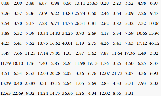
The data has been used by Kumar et al. [25], El-Gohary et al. [26], Chandra [27], De Andrade and Zea [28] and Selim [29].

We fitted the above-mentioned data sets using MLE to the flexible reduced logarithmic-inverse Lomax (FRL-IL), inverse Nadarajah-Haghighi (INH), inverse Weibull (IW), inverse exponential (IE) and Inverse Generalized Power Weibull IGPW distributions. The MLEs for IGPW, INH, IW, IE and FRL-IL distributions are displayed in Table 1. Kolmogorov-Smirnov (K-S), -Log likelihood (-L), Akaike Information Criterion (AIC), Consistent Akaike Information Criterion (CAIC), Bayesian Information Criterion (BIC) and Hannan-Quinn Information Criterion (HQIC) were used to compare the fitted models. Based on these criteria, the best model is the one that achieves the lowest values for the information criteria and goodness-of-fit statistics. Hence, it is clear from the numerical results in Table 2, The FRL-IL model presents a better fit than other compared models. Figure 7 displays the empirical and fitted cumulative for the FRL-IL.

Also, Figure 7 graphically illustrates that FRL-IL distribution provides the best fit to our data sets, as compared to the other considered models. Therefore, the FRL-IL model can be used as a possible alternative to the well-known models

Figure 7. The empirical and fitted for the FRL-IL.

Table 1. The estimates $\alpha ,\beta$ and $\lambda$.

Table 2. The estimates of the goodness-of-fit for data

like inverse exponential and inverse Weibull models.

7. Conclusion

This paper presents a new three-parameter distribution, called the flexible reduced logarithmic-inverse Lomax distribution. Some of the statistical properties of the (FRL-IL) distribution include the moments, hazard rate function, quantile function and order statistics are derived. To estimate the model parameters, the maximum likelihood approach is used. The practical applications have established that the proposed distribution is quite useful for dealing with reliable data and behaves better. Also, the figure graphically illustrates that FRL-IL distribution provides the best fit to our data sets, as compared with the other considered models. Therefore, the FRL-IL model can be used as a possible alternative to the well-known models like inverse exponential and inverse Weibull models. In the future, it will be developed and studied the generalized FRL-IL distribution under progressively type II and hyper type II censored.

Conflicts of Interest

The authors declare no conflicts of interest regarding the publication of this paper.

References

[1]	Lomax, K.S. (1954) Business Failures: Another Example of the Analysis of Failure Data. Journal of the American Statistical Association, 49, 847-852. https://doi.org/10.1080/01621459.1954.10501239
[2]	Hassan, A. and Al-Ghamdi, A. (2009) Optimum Step Stress Accelerated Life Testing for Lomax Distribution. Journal of Applied Sciences Research, 5, 2153-2164.
[3]	Corbellini, A. Crosato, L. Ganugi, P. and Mazzoli, M. (2009) Fitting Pareto II Distribution on Firm Size: Statistical Methodology and Economic Puzzles. In: Skiadas, C., Ed., Advances in Data Analysis. Statistics for Industry and Technology. Birkhäuser, Boston. https://doi.org/10.1007/978-0-8176-4799-5_26
[4]	Bryson, M. (1974) Heavy-Tailed Distributions: Properties and Tests. Technometrics, 16, 61-68. https://doi.org/10.1080/00401706.1974.10489150
[5]	Kleiber, C. (2004) Lorenz Ordering of Order Statistics from Log-Logistic and Related Distributions. Journal of Statistical Planning and Inference, 120, 13-19. https://doi.org/10.1016/S0378-3758(02)00495-0
[6]	Yadav, A.S., Singh, S.K. and Singh, U. (2018) Bayesian Estimation of Lomax Distribution under Type-II Hybrid Censored Data Using Lindley’s Approximation Method. International Journal of Data Science, 2, No. 4. https://doi.org/10.1504/IJDS.2017.10009048
[7]	Rahman, J., Aslam, M. and Sajid, A. (2013) Estimation and Prediction of Inverse Lomax Model via Bayesian Approach. Caspian Journal of Applied Sciences Research, 2, 43-56.
[8]	Singh, S.K. and Singh, U. (2016) Reliability Estimation for Inverse Lomax Distribution under Type II Censored Data Using Markov Chain Monte Carlo Method. International Journal of Mathematics and Statistics, 17, 128-146.
[9]	Reyad, H.M. and Othman, S.A. (2018) E-Bayesian Estimation of Two-Component Mixture of Inverse Lomax Distribution Based on Type-I Censoring Scheme. Journal of Advances in Mathematics and Computer Science, 26, 1-22. https://doi.org/10.9734/JAMCS/2018/39087
[10]	Rama, S. and Kamlesh Kumar, S. (2019) A Generalization of Generalized Gamma Distribution. International Journal of Computational and Theoretical Statistics, 6, 33-42. https://doi.org/10.12785/ijcts/060105
[11]	Oluyede, B. (2018) The Gamma-Weibull-G Family of Distributions with Applications. Austrian Journal of Statistics, 47, 45-76. https://doi.org/10.17713/ajs.v47i1.155
[12]	Maiti, S. and Pramanik, S. (2019) Odds XGamma-G Family of Distributions. IAPQR Transactions, 43, 135-163. https://doi.org/10.32381/IAPQRT.2019.43.02.3
[13]	Korkmaz, M.C., Alizadeh, M., Yousof, H.M. and Butt, N.S. (2018) The Generalized Odd Weibull Generated Family of Distributions: Statistical Properties and Applications. Pakistan Journal of Statistics and Operation Research, 14, 541-556. https://doi.org/10.18187/pjsor.v14i3.2598
[14]	Aslam, M., Asghar, Z., Hussain, Z. and Shah, S.F. (2020) A Modified TX Family of Distributions: Classical and Bayesian Analysis. Journal of Taibah University for Science, 14, 254-264. https://doi.org/10.1080/16583655.2020.1732642
[15]	Gallardo, D.I., Gomez, Y.M., Gomez, H.W. and de Castro, M. (2020) On the Use of the Modified Power Series Family of Distributions in a Cure Rate Model Context. Statistical Methods in Medical Research, 29, 1831-1845. https://doi.org/10.1177%2F0962280219876962
[16]	Al-Saiary, Z.A. and Bakoban, R.A. (2020) The Topp-Leone Generalized Inverted Exponential Distribution with Real Data Applications. Entropy, 22, Article No. 1144. https://doi.org/10.3390/e22101144
[17]	Bantan, R.A., Jamal, F., Chesneau, C. and Elgarhy, M. (2020) Type II Power Topp-Leone Generated Family of Distributions with Statistical Inference and Applications. Symmetry, 12, Article No. 75. https://doi.org/10.3390/sym12010075
[18]	Al-Babtain, A.A., Elbatal, I., Chesneau, C. and Elgarhy, M. (2020) Sine Topp-Leone-G family of Distributions: Theory and Applications. Open Physics, 18, 574-593. https://doi.org/10.1515/phys-2020-0180
[19]	Al-Babtain, A.A., Elbatal, I., Chesneau, C. and Jamal, F. (2020) Box-Cox Gamma-G Family of Distributions: Theory and Applications. Mathematics, 8, Article No. 1801. https://doi.org/10.3390/math8101801
[20]	Liu, Y., Ilyas, M., Khosa, S.K., Muhmoudi, E., Ahmad, Z., Khan, D.M. and Hamedani, G.G. (2020) A Flexible Reduced Logarithmic-X Family of Distributions with Biomedical Analysis. Computational and Mathematical Methods in Medicine, 2020, Article ID: 4373595. https://doi.org/10.1155/2020/4373595
[21]	Kenney, J. and Keeping, E. (1962) Mathematics of Statistics. Vol. 1, Nostrand Company, Princeton.
[22]	Moors, J.J.A. (1998) A Quantile Alternative for Kurtosis. The Statistician, 37, 25-32. https://doi.org/10.2307/2348376
[23]	Lawless, J.F. (2011) Statistical Models and Methods for Lifetime Data. John Wiley and Sons, New York, 362.
[24]	Lee, E.T. and Wang, J. (2003) Statistical Methods for Survival Data Analysis. John Wiley and Sons, 476. https://doi.org/10.1002/0471458546
[25]	Kumar, D., Singh, U. and Singh, S.K. (2015) A Method of Proposing New Distribution and Its Application to Bladder Cancer Patients Data. Journal of Statistics Applications and Probability Letters, 2, 235-245.
[26]	El-Gohary, A., El-Bassiouny, A. and El-Morshedy, M. (2015) Inverse Flexible Weibull Extension Distribution. International Journal of Computer Applications, 115, 46-51. https://doi.org/10.5120/20127-2211
[27]	Chandra, N. and Sen, S. (2017) The Quasi Xgamma Distribution with Application in Bladder Cancer Data. Journal of Data Science, 15, 61-76. https://doi.org/10.6339/JDS.201701_15(1).0004
[28]	De Andrade, T.A. and Zea, L.M. (2018) The Exponentiated Generalized Extended Pareto Distribution. Journal of Data Science, 16, 781-800. https://doi.org/10.6339/JDS.201810_16(4).00007
[29]	Selim, M.A. (2019) Some Theoretical and Computational Aspects of the Inverse Generalized Power Weibull Distribution. Journal of Data Science, 17, 742-755. https://doi.org/10.6339/JDS.201910_17(4).0007