The Distribution of Multiple Shot Noise Process and Its Integral ()
Increases in the frequency and intensity of storms, hail, bushfires and earthquakes have revealed shortcomings in the ways Catastrophe Insurance is priced. Hence more complicated models are needed to accommodate increasing frequency and intensity of catastrophic events. A Cox process with shot noise intensity has been suggested to use to predict claims arising from catastrophic events by Dassios and Jang [2].
In financial industry, a shock which initially affects a couple of institutions or a particular region of the economy spreads to the rest of the financial industry and then infects the larger economy. This is called “financial contagion” [4,5]. The US federal takeover of Fannie Mae and Freddie Mac, the Bank of America takeover of Countrywide Financial Corporation and the bankruptcy of New Century Financial Corporation due to mismanagement of subprime mortgage in US are the examples of financial contagion. The prevalence of above financial contagion has led to further bankruptcies and default of mortgage lenders in US announcing their significant losses in 2008. This subprime mortgage meltdown has also led to new ownership for Bears Stern and Merrill Lynch and the bankruptcy of Lehman Brothers. These contagious events have caused the collapse of stock prices in worldwide and it has shaken global financial markets further due to new waves of default and bankruptcy. Due to the failing of financial institutions in 2008, systemic risk has become the main concern to the governments requiring their interventions to ameliorate these contagious effects to the larger economy [6].
To these effects, in this paper we introduce multiple shot noise process [7]. It consists of  component
processes ,
,  ,
,  ,
, 
 where each process acts as a jump intensity for the next one. For

 decays with rate
 , and additive jumps occur with rate of
 , i.e. each
process acts as a jump intensity for the next one. Jump sizes are independent but not identically distributed
random variables with distribution function 
 decays with rate
  but its jump arrival rate
is deterministic . Its jump sizes have distribution function
  Hence multiple shot noise process we consider has the following structure:
 (1)
(1)
where:
・  are sequences of independent but not identically distributed random
variables with distribution function 
 and
and 
・ ![]() is the total number of events up to time
is the total number of events up to time ![]()
・ ![]() is the rate of exponential decay for the firm
is the rate of exponential decay for the firm ![]()
We also make the additional assumption that the point process ![]() and the sequences
and the sequences ![]() are independent of each other.
are independent of each other.
![]() follows a homogeneous Poisson process with frequency rate
follows a homogeneous Poisson process with frequency rate ![]() and
and ![]() for
for ![]() follows a Cox process with intensity rate
follows a Cox process with intensity rate![]() , respectively [8-10]. So in this model, dependence between the processes
, respectively [8-10]. So in this model, dependence between the processes ![]() comes from the structure that each process acts as a jump intensity for the next one.
comes from the structure that each process acts as a jump intensity for the next one.
The process  is triggered by jumps (or primary events, or shocks) that will result in a positive jump in the process. As time passes, the process decreases with rate
  until another jump (or event) occurs which again will result in a positive jump in the process. The process
  is the jump arrival rate for the
  process
 , and the process
  is the jump arrival rate for the
  process
 , and so on. Hence the process
  is the prime trigger in influencing all other relative processes. As time passes, the processes
  decrease with rate
  for
for , and additive jumps occur.
We use another Cox process  for
for  to model the multivariate jump time and derive the tail of multivariate distribution of the first jump times of the Cox processes, i.e. the multivariate survival function, where it is assumed that the jumps in
  for
for , the jumps in
  for
for  and primary event jumps in
  are independent of each other.
If  (i.e.
(i.e. ), this process becomes a double shot noise process, and it can be considered to model the level of water in dams and rivers using this process. Applying a double shot noise process in insurance context can be noticed in Dassios and Jang [11].
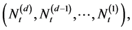
In Section 2, we start with deriving the Laplace transform of the vector

using the martingale methodology in Dassios and Jang [2], with which we obtain the expression for
 (1.2)
(1.2)
where  and
and  for
for  For simplicity, it is assumed that
  but it
can be easily extended to the higher dimensions. Using (1.2) in Section 3, we derive the tail of the multivariate
distribution of ’s, where
 , i.e.
 (1.3)
(1.3)
that is equivalent to the first jump time of the Cox process . The expressions for relevant multivariate distributions such as
 (1.4)
(1.4)
and
 (1.5)
(1.5)
are omitted as they can easily be obtained using (1.2) and (1.3), but their numerical calculations are shown in Section 4. Section 5 contains some concluding remarks.
2. The Laplace Transform of the Vector 
We firstly consider using the Laplace transform of the vector

to derive the tail of the multivariate distribution of ’s. Once its expression is obtained, we can easily derive the tail of the multivariate distribution of
 ’s by setting
 in the Equation (1.2).
With the aid of piecewise deterministic Markov process theory and using the results in [1], the infinitesimal
generator of the process  acting on a function
 within its domain
  is given by
 (2.1)
(2.1)
For  to belong to the domain of the generator
 , it is sufficient
that  is differentiable w.r.t.
 ,
,  for all
 ,
,  ,
,  and that

We assume that the Cox processes jumps, intensity jumps and primary event jumps do not occur at the same time.
Let us find a suitable martingale to derive the Laplace transform of the vector , the
, the
Laplace transform of the vector  and the p.g.f. (probability generating function) of the vector
 respectively.
Theorem 2.1 Considering constants ,
,  and
and  such that
 ,
,  and
and 
 (2.2)
(2.2)
is a martingale, where
and

where

Proof. From (2.1),  has to satisfy
  for it to be a martin-
gale. Setting

we get the Equation
 (2.3)
(2.3)
from which we have


Solve these Equations, then the result follows.
For simplicity, we set  (i.e.
(i.e.  and 1), but it can be easily extended to the higher dimension cases.
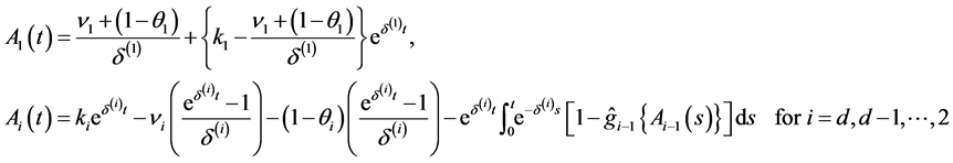
Theorem 2.2 Let  be as defined. Then
 (2.4)
(2.4)
where
![]()
![]()
![]()
![]()
and ![]()
![]() for
for![]() .
.
Proof. Using the martingale derived in Theorem 2.1, we have
![]() (2.5)
(2.5)
Hence the result follows immediately if we set
![]()
![]()
and
![]()
in (2.5).
Corollary 2.3 Let![]() ,
, ![]() and
and ![]() be as defined for
be as defined for ![]() and 1. Then
and 1. Then
![]() (2.6)
(2.6)
and
![]() (2.7)
(2.7)
Proof. If we set ![]() in (2.4), (2.6) follows. If we also set
in (2.4), (2.6) follows. If we also set ![]() in (2.4), (2.7) follows.
in (2.4), (2.7) follows.
Now we can easily derive the Laplace transform of the vector ![]() the Laplace transform of the
the Laplace transform of the
vector ![]() and the p.g.f. of the vector
and the p.g.f. of the vector![]() , respectively.
, respectively.
Corollary 2.4 The Laplace transform of the vector ![]() and the Laplace transform of the vector
and the Laplace transform of the vector ![]() are given by
are given by
![]() (2.8)
(2.8)
![]() (2.9)
(2.9)
and the p.g.f. of the vector ![]() is given by
is given by
![]() (2.10)
(2.10)
Proof. If we set ![]() in (2.6) and (2.7) respectively, (2.8) and (2.10) follow. If we also set
in (2.6) and (2.7) respectively, (2.8) and (2.10) follow. If we also set ![]() in (2.6) or set
in (2.6) or set ![]() in (2.7), (2.9) follows.
in (2.7), (2.9) follows.
Remark 1: It would be interesting to apply the p.g.f. of the vector ![]() to model insurance claim arrivals as well as the number of losses to the entire financial system/market. Also using (2.10), the marginal probability generating function for the number of jump can be easily derived. The derivation of the
to model insurance claim arrivals as well as the number of losses to the entire financial system/market. Also using (2.10), the marginal probability generating function for the number of jump can be easily derived. The derivation of the
marginal probability generating function for ![]() and its usage in insurance context can be
and its usage in insurance context can be
found in Dassios and Jang [2,12]. To obtain the mean and variance of the level of water in dams and rivers, the
Laplace transform of the vector![]() , i.e.
, i.e. ![]() can be also used.
can be also used.
Corollary 2.5 The Laplace transform of the vector![]() , where
, where![]() ,
, ![]() and
and ![]() are jointly stationary is given by
are jointly stationary is given by
![]() (2.11)
(2.11)
Proof. Let ![]() in (2.9) and the result follows.
in (2.9) and the result follows.
3. Multivariate Survival Function
Having derived the Laplace transform of the vector ![]() and the Laplace transform of the vector
and the Laplace transform of the vector ![]() in the previous section, we can easily obtain the tail of multivariate distributions of the first jump times of the Cox processes (i.e. the multivariate survival function), other relevant joint distributions and the marginal survival functions. To do so, we start with a corollary assuming that
in the previous section, we can easily obtain the tail of multivariate distributions of the first jump times of the Cox processes (i.e. the multivariate survival function), other relevant joint distributions and the marginal survival functions. To do so, we start with a corollary assuming that![]() ,
, ![]() and
and ![]() are jointly stationary.
are jointly stationary.
Corollary 3.1 The Laplace transform of the vector ![]() where
where![]() ,
, ![]() and
and ![]() are jointly stationary, is given by
are jointly stationary, is given by
![]() (3.1)
(3.1)
Proof. Take the expectation to (2.8) and use (2.11), then (3.1) follows.
Now, we can obtain the multivariate survival function, other relevant joint distributions and the marginal survival functions.
Corollary 3.2 The multivariate survival function, where![]() ,
, ![]() and
and ![]() are jointly stationary, is given by
are jointly stationary, is given by
![]() (3.2)
(3.2)
Proof. If we set ![]() in (3.1), (3.2) follows immediately.
in (3.1), (3.2) follows immediately.
Using (3.2), we can obtain other relevant joint distributions, three bivariate survival functions, i.e.
![]()
and other relevant bivariate distributions. We can also obtain three marginal survival functions, i.e.
![]()
They are omitted as they can easily be obtained by using the values for the vector ![]() with 0 or 1 in (3.1). Instead, we present numerical calculations of eight joint distributions with these survival functions in Section 4.
with 0 or 1 in (3.1). Instead, we present numerical calculations of eight joint distributions with these survival functions in Section 4.
4. Numerical Examples
In this section, we show the calculations of multivariate survival function, other relevant joint distributions and the survival functions, i.e. eight joint distributions, three bivariate survival functions and three marginal survival functions. To do so, we use three exponential distributions for jump sizes for![]() ,
, ![]() and
and![]() , respectively, which are:
, respectively, which are:
![]() (4.1)
(4.1)
Other distributions such as normal, log-normal, gamma and Pareto, etc. can be also applied for jump size distributions for ![]() (
(![]() and 1).
and 1).
Using (3.2), one of corresponding bivariate survival functions is given by
![]() (14)
(14)
We can easily obtain other corresponding bivariate survival functions, i.e.
![]()
which are omitted as they have similar nested expressions to (4.2).
Using (3.2), one of corresponding marginal survival functions is given by
![]() (4.3)
(4.3)
which can be found in Dassios and Jang [2]. We can also find another corresponding marginal survival function, i.e.
![]() (4.4)
(4.4)
We can easily obtain remaining marginal survival function, i.e. ![]() which are omitted as it has also similar extended nested expressions to (4.4).
which are omitted as it has also similar extended nested expressions to (4.4).
Now let us illustrate the calculations of three marginal survival functions, three bivariate survival functions and eight joint distributions. To do so, we use the parameter values as below:
![]() (4.5)
(4.5)
Example 4.1 (Marginal survival functions)
The calculations of three marginal survival functions, i.e.
![]()
are given by
![]()
Example 4.2 (Bivariate survival functions)
The calculations of three bivariate survival functions, i.e.
![]()
are given by
![]()
Example 4.3 (Eight joint distributions)
The calculations of eight joint distributions, i.e.
![]()
are given by
![]()
![]()
![]()
![]()
![]()
![]()
![]()
![]()
Remark 2: Example 4.1 shows that the survival probability of the firm 1 is the highest and the firm 2’s and the firm 3’s, which can be modified with different parameter values for (4.5). Example 4.2 and 4.3 show that all relevant joint probabilities are in line with each survival probability in Example 4.1. For example, the joint survival probability of firm 2 and 1, ![]() is the highest as the combination of these two firms’ survival probabilities are the highest. Also it can be easily noticed that
is the highest as the combination of these two firms’ survival probabilities are the highest. Also it can be easily noticed that ![]() is the highest in Example 4.3 as the joint survival probability of firm 2 and 1 is the highest.
is the highest in Example 4.3 as the joint survival probability of firm 2 and 1 is the highest.
An economic interpretation from the perspective of the multiple shot noise process is the following. After the firm 3 ceases to function (e.g. default of Lehman Brothers), its intensity is still around affecting the other firms in the way of the multiple shot noise process. Hence ![]() can be interpreted as the probability that the firm 2 and 1 survive together after the firm 3 ceases to function, but its intensity is still in action. Also
can be interpreted as the probability that the firm 2 and 1 survive together after the firm 3 ceases to function, but its intensity is still in action. Also ![]() can be interpreted as the probability that the firm 1 survives after the firm 3 and 2 cease to function, but their intensities are still in action.
can be interpreted as the probability that the firm 1 survives after the firm 3 and 2 cease to function, but their intensities are still in action.
After the failing of the firm 3, ![]() can be considered as a measure to decide whether the government’s intervention is required not to fail the firm 2 and 1 with a threshold probability (e.g. 0.5) assumng that its intensity is still in action. Also by simulating the multiple shot noise process, this probability can be easily obtained as a systemic risk management tool for the governments.
can be considered as a measure to decide whether the government’s intervention is required not to fail the firm 2 and 1 with a threshold probability (e.g. 0.5) assumng that its intensity is still in action. Also by simulating the multiple shot noise process, this probability can be easily obtained as a systemic risk management tool for the governments.
5. Conclusions
We introduced multiple shot noise process, where each process acts as a jump intensity for the next one, and its integral. These two processes can be used in hydropower, dam and river engineering fields. Based on the piecewise deterministic Markov process theory developed by Davis [1] and the martingale methodology used by Dassios and Jang [2], we derived the Laplace transforms of these two processes. Using the multivariate Cox process, the multivariate probability generating function for the number of jumps was also presented. To do so, we have made an assumption that the Cox processes jumps, intensity jumps and primary event jumps are independent of each other. This probability generating function can be considered applying to modeling insurance claim arrivals as well as the number of losses to the entire financial system/market.
Using the Laplace transform of the integral of multiple shot noise process, we obtained the tail of multivariate distributions of the first jump times of the Cox processes, i.e. the multivariate survival functions. These survival functions can be used as the measures to decide whether the government intervention is required to ameliorate the contagious effects to the entire financial system or larger economy. With exponential distributions for jump sizes, we calculated multivariate survival function, other relevant joint distributions and the survival functions. We leave the applications of what we presented in this paper, i.e. a multivariate Cox process with multiple shot noise intensity, multiple shot noise process and its integral to the fields mentioned above for further research.