Application of Continous Time Model in Prediction of Loss Reserves in Credit Insurance for Asset-Based Lending Companies ()
1. Introduction
Credit Insurance is used to pay out a loan balance or to postpone debt payments on the customer’s behalf in the event of disability or job loss. Credit insurance can be purchased to insure all kinds of consumer loans including car loans, loans from finance companies, and home mortgage borrowing. Credit insurance is as a result of credit risk. In this paper, we model credit risk and estimate default probabilities which will help us come up with the final reserve. [1] investigated the default probabilities and their comparative statics (default Greeks) in the Merton framework using the objective or real probability measure. [2] used Black-Scholes formula for European call option to find the probability of default of a firm. In their paper, they also describe the factors that affect the default probability using Black-Scholes model for European call option by the help of some examples. Structural models pioneered by [3] employ modern option pricing theory in corporate debt valuation. Merton model Black and Scholes was the first structural model and has served as the cornerstone for all other structural models. Structural approach, led by Merton model has a very nice feature of connecting credit risk to underlying structural variables. It provides both an intuitive economic interpretation and an endogenous explanation of credit defaults, and allows for applications of option pricing methods. As a result, structural models not only facilitate security valuation, but also address the choice of financial structure. In 1973, Merton developed the contingent claims model that provides the motivation for the behavior of the borrower using the options theory Black and Scholes. Most studies initially used this approach in the valuation of mortgages by focusing on default and prepayment as individual risks. For example, [4] used the Black-Scholes option-pricing model to value the risk of default by considering the default risk as a put option sold by the FHA and purchased by the buyer of a home for the protection of risk of default to the lender. [5] presented the idea of hedging and pricing by arbitrage in the discrete-time setting by binary trees. The key probabilistic concepts of conditional expectation, martingales, change of probability measure and representation are all introduced. They also presented the concepts of expectation pricing versus arbitrage. [5] also brought to table the idea of hedging and pricing by arbitrage in the continuous time setting. Brownian motion is brought out as well as the Itô calculus needed to manipulate it culminating in a derivation of the Black Scholes formula. Pricing of an individual asset subject to credit risk has been extensively studied in the literature we refer to [6] for the survey of such pricing models. They proposed another model in which the payoffs are discounted by an interest rate that is adjusted so as to reflect the effect of default risk. Among them, [7] assumed that the payoffs upon default are expressed as an exogenous fraction of the claim and they showed, under some regularity conditions, the price is given by the expected discounted payoffs under the risk neutral probability measure. The Health-Jarrow-Morton type model of defaultable term structures with multiple ratings was proposed by [8] and [9] . Bardhan et al., (2006) in their Journal of Real Estate Finance and economics [10] developed a new option-based method for valuation of mortgage insurance contracts in closed economy where agents are risk neutral. As an application, they priced a typical Serbian government backed mortgage insurance contract. [11] used the concept of Geometric Brownian to describe the random behaviour of the asset price St over time. In our case, we examine the random behaviour of the delinquency index Yt.
Asset-based lending companies and other loan providers are exposed to risk of loan defaults by borrowers. To lessen this risk, these companies acquire credit insurance. Therefore when the borrower defaults in his or her credit payment, the insurance company covers a percentage of the outstanding balance and the rest of the balance is taken care of by the insured lender through repossession of the collateral. Although data might be available, the pricing of credit insurance for asset based lending companies is a challenging task and is even more challenging in the case of emerging markets like Kenya, where, in the case of a borrower’s default, the process of repossession of loan collateral may last a longer period of time of more than a year and where data on payment behavior is generally unavailable or of poor quality. The current valuation methods do not consider the time to repossession of an asset in case of loan default.
In this paper we propose a continuous time (Black-Sholes) model to forecast loss reserves in credit insurance for asset-based lending companies. This model takes into account the time to repossession of the collateral which is not accounted for in frequency severity and hazard rate models.
Instead of replacing currently used models, this will also present an alternative method for insurers looking for a reasonable check for their reserves and premiums levels. Our proposed projection techniques can be applied in any market, especially in emerging market economies where other existing methods may be either unsuitable or are too difficult to use due to inadequate significant data.
Using our continuous time model, all insurers in Kenya even those with absence of resident Actuaries can use historical data from existing insurers and their office experience data to accurately value credit insurance contracts. This will in turn grow the number of credit insurance companies hence bringing forward healthy competition and improved services. Financial institutions will be protected from the risk of loan defaults.
Oscar Perez et al., in his study, applied Stochastic Calculus techniques to estimate loss reserves in mortgage insurance. He focused on mortgage backed securities in Mexico [12] .
In this study, we extensively extend this knowledge to valuation in credit insurance for the case of asset-based lending companies.
2. Methodology
2.1. Credit Risk Modeling
Here, we model credit risk and present Insurance function in order to obtain the expected present value of the payments of the Insurance. This will be done by applying the binomial model (discrete model). Consider a borrower with a loan term of N months given by a financial institution. Let a stochastic process Y represent the number of defaultable periods (delinquency index) as of time t. Then,
Under certain circumstances, the value of Yt can be negative. In such scenarios we treat Y as absolute value. Let pi represent the probability that the borrower fails to make his credit payment for time i. Denote a function
which is a function that depends on the delinquency index. Consider cash bond Bt to be another stochastic process to represent the time-value of money. Assume a constant risk-free rate r. Thus
with condition that B0 = 1. We thus analyze the simple case of the process Yt by applying binomial trees. That is, when N = 1 we can represent the compensation by the insurer
of the delinquency index at time 1 as follows:
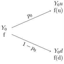
From the above figure, we can obtain the expected present value of the compensation by the insurance using the following formula:
(2.1)
where;
represents compensation paid by an Insurance company in which the borrower defaults payment; and
represents compensation paid by an Insurance company in which the borrower pay the corresponding payment of his credit.
Thus by Kolmogorov’s strong law of large numbers, if the insurance company has a large number of portfolio, then that company can expect a loss given by formula (2.1).
2.2. Generalization of the Binomial Model
We use the binomial tree of two steps to generalize the binomial model. In this case we will do our analyzation by considering the case when N = 2, (t = 0, 1, 2) under the probability measures
and
.
Where N is the loan term.
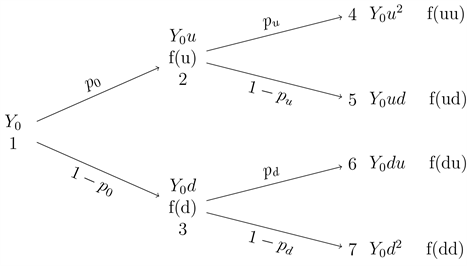
Based on the diagram above we can name the outcomes of the delinquency index and its proportion of upward and downward movement based on the path followed by the process, for example, ud shows the outcome when the process had an upward movement in the first time and then a downward movement in the second step.
In our generalization and considering the methods in the previous section, we can calculate the expected present value of the possible losses of the insurance company which issues f(.) as follows. At time 0, we can estimate the expected present value of the losses of the company at time as follows;
(2.2)
We now apply the method of replicating asset portfolio in order to make change of probability measure. This enables us find another way of expressing the expected present value of the losses to the insurance company.
Suppose an insurance company wishes to match its losses by using the following portfolio:
where A(Yt) is an asset whose value depends on the delinquency index Yt and Bt is a cash bond that has the risk-free rate r.
Then the above portfolio Ct should replicate the losses of the insurance company. Thus we have;
(2.3)
From Equation (2.2) we have;
(i)
and
(ii)
solving Equations (i) and (ii) simultaneously, we obtain;
where;
is the filtration at time t when in the last path of that filtration there was a rise in the value of the delinquency index, and
is the filtration at time t when in the last step of that filtration there was a decrease in the value of the delinquency index. If we substitute at and bt in Ct we obtain:
We thus can be able to change the probability measure from
to
and the following is now the generalization of the results.
This is a very significant result that will be used in the following section.
2.3. The Continuous Model
2.3.1. Brownian Motion
Let’s modify the binomial tree shown in the previous sections. If we take changes
in time to correspond to
where N is the term of the loan (asset-based) and suppose that the borrower can increase or decrease its “delinquency index”
with probability
. Let xi be a random variable:
Therefore the delinquency index at time t can be written down as:
Based on the central limit theorem:
.
The unconditional probability density function which follows
at a fixed time t for Wiener process (Brownian Motion process) is given by;
The expectation is zero,
Thus
2.3.2. Geometric Brownian Motion
It’s a continuous time stochastic process in which the logarithm of the randomly varying quantity follows a Brownian Motion with drift. Thus a stochastic process is said to follow a Geometric Brownian Motion if it satisfies the following stochastic differential equation;
where
is a Wiener process (Brownian Motion) and (
the drift) and (
the volatility) are constants. The expression of this diffusion is
(2.4)
We can solve this stochastic differential Equation (2.4) by applying Itô’s lemma (shown below); This model is very important in the formulas developed further.
2.3.3. Itô’s Lemma
Assume that Y has a stochastic differential given by
(2.5)
where
and
are adapted processes. Define the process Z by
. Then Z has a stochastic differential given by
(2.6)
Proof. Taking Taylor expansion including second order terms, we obtain;
Squaring Equation (2.5) we obtain;
(2.7)
Substituting Equation (2.5) and (2.7) into the Taylor expansion taking into account the following conditions,
We obtain the result (2.6). □
We can obtain the solution to the Geometric Brownian Motion SDE shown above by applying Itô’s lemma as follows;
(2.8)
(2.9)
where
is the quadratic variation of the SDE
Assuming;
Thus
.
Substituting the value of
and
in Equation (2.9) we obtain;
Written in the integral form, this leads to
Thus this equation can also be written as;
(2.10)
2.4. Credit Insurance and Reserving
In this study we are looking at credit insurance in the case of asset-based lending where a borrower borrows money to buy a car. Thus the definition for credit insurance becomes; a financial tool for transferring credit risk of a credit from a financial institution to an insurance company. The financial institution has to pay a premium and the insurance company will pay a percentage of the outstanding balance of the loan plus interests if there is a default. In this case Credit insurance will pay the benefit only when the borrower defaults in their payments and the financial institution takes over or recover the underlying car (collateral) for that loan.
Therefore if we denote the loss reserve at time t as OCRt, X the random variable representing the losses, and
the filtration of the delinquency index we can write
We can say that this OCRt exhibits markovian property. We can build it further in the following sections.
2.5. Black-Scholes Estimations
Assume that the delinquency index can be modeled as a geometric Brownian motion, we will have;
(2.11)
(2.12)
Consider cash bond Bt as the stochastic process that give the risk-free rate, that is:
(2.13)
Rememeber we need an asset that depends on the delinquency index whose present value is a martingale. Denote that asset as A(Yt) and we suppose that its linearly proportional to the delinquency index as follows;
Let’s also denote D = (Dt) t ≥ 0 to be the stochastic process representing the present value of At:
when we apply ltô’s lemma to Dt we get:
(2.14)
Proof. Recall that
(2.15)
But
.
Thus Equation (2.15) becomes;
□
Based on the construction of asset portfolio strategy we were able to make change of probability measure. This implied the present value of the asset which depends on the delinquency index was a martingale. Therefore, we will make a change in probability measure from
to
on the process Dt in order to make Dt to be a martingale. Based on the Cameron-Martin-Girsanov theorem, for each probability measure
equivalent to
and if we have a previsible process
then:
is also
Brownian motion with
.
Substituting in (2.14) we have:
for Dt be a martingale we need
since drift equals 0. The solution of this equation is the Market price of risk;
(2.16)
But Dt is a martingale;
(2.17)
Considering the concepts shown so far, the delinquency index under the probability measure
is:
Proof. Recall
(2.18)
But
and from
Thus Equation (2.17) becomes
as above. □
Thus under the probability measure
the drift of the delinquency index is the risk-free rate. Solving this stochastic differential equation, we can have estimate of the delinquency index;
(2.19)
This is an important result which will enable us forecast future losses of a credit insurance which pays f(T):
(2.20)
where:
OCRt is the reserve at time t given information of the filtration
.
Bt = Is cash bond which give the risk-free rate r.
and
.
f(T) = Is the compensation by the insurance company. T is the random variable that represents the time to paying the sum insured. Remember, the credit insurance pays claims when the car is taken over. In the case the outstanding loan balance upon default is more than the value of the collateral, the insured lender will exercise the right to sell the collateral at the outstanding loan balance. This is achieved by the lender receiving from the insurer the difference of the outstanding loan and the market value of the car at the time of default. The contract is therefore settled by the difference.
In this case, the total cost of the policy holder will be the premium paid and the value of the collateral upon default. In addition to the time of valuation, t we must consider another random variable u representing the time to repossession of the car and thus T = t + u as denoted above.
The time to repossess a car is not certain, it can take more than a year. That’s why we use the random variable u. Moreover, the financial institutions which insure itself with the insurance company have delays in giving out the information of the delinquency index and this gives the reason for use of t0 which is about one month or two. Based on these reasons, we are going to forecast the future losses of credit insurance at time t, with the information given by the financial institution at time t0 with the filtration
. We can see that
. Consider t0 to be independent of t, we can develop Equation (2.19). Consider f(T) to be the function that represents compensation by the insurance company (assuming that the car is recovered after R months defaultable period). It will be defined as a percentage of the outstanding balance at time of recovering the car if the delinquency index is greater than R. Where R is the delinquency index threshold. That is:
%Cov = Is the percentage of the covered outstanding balance by the insurance company.
= Is the outstanding balance of the credit at time T.R is the delinquency index threshold.
= Is an indicative random variable:
Then, we have;
Since
is modelled as Geometric Brownian motion, it conforms to a diffusion process, and it thus possess the Markovian property. Consequently we can reorganize the terms in the above equation as:
(2.21)
(2.22)
Since
is a Geometric Brownian Motion, we have;
Taking the notation of the Black-Scholes we have;
captures the idea of credit risk in the Merton Model. It denotes the probability of default. Formula (2.22) turns into:
(2.23)
We thus have managed to obtain the formula to forecast loss reserves in credit insurance if we know just the percentage of outstanding balance covered by the insurer, the value of the delinquency index, a risk-free rate, and the distribution of the random variable u. We can write Equation (2.23) as:
(2.24)
where:
p(u) is the probability density function of u.
n is the loan term.
is the outstanding balance of the loan at time t plus interest at the rate c:
We can simplify this calculation by taking u as a constant:
(2.25)
Since this formula was obtained under the probability measure
we have a replicating portfolio
, which matches the future losses of the insurance company. Thus:
(2.26)
(2.27)
where;
denotes number of units of
.
denotes number of units of the cash bond. Let
be the process representing the present value of the portfolio:
(2.28)
Considering the following equation and applying Itô’s lemma we have;
can be obtained from (2.28). We’ve therefore found an alternative method for projecting losses in credit insurance products and a replicating portfolio to match them.
3. Main Results
We simulated the outstanding balances of 30 loanees by considering a case where we can have a car loan business with assets valued between 1 million and 10 million. We did this so that we can be able to explain our model. The result of the future loss was estimated by considering the following assumptions (Table 1).
u is a random variable representing the time to recover the collateral while c is a simple interest and t is the time of valuation. Since most car loan businesses have a loan term of 5 years, we assumed this in our estimation (Table 2).
![]()
Table 1. Table showing the assumed constants.
![]()
Table 2. Estimates of the delinquency index (Yt).
The estimates of the delinquency index were estimated as follows: (Table 2)
d2 was obtained using the following formula: (Table 3)
The
was obtained as:
(Table 4).
An increase in the value of the probability of default increases the value of the reserve estimated depending on the value of the outstanding balance of the borrower. We can therefore deduce that a borrower with higher chances of default will make the insurance company to have longer reserve requirements. Despite this, it’s also possible to have shorter reserve requirements. This means that a borrower with lower chances of default, will result to lower levels of reserve (see Figure 1). An increase in the loan term or the time to maturity of the payment of the insurance has the effect of reducing the probability of default by the borrower. This will result to shorter reserve requirements by the insurance company.
The number of defaultable periods (delinquency index) has the effect of increasing the estimate of future reserve by the insurance company. Therefore if an insurance company insures policies with a large number of defaultable periods, it will have longer reserve requirements otherwise it will have shorter reserve requirement (see Figure 2).
A longer loan term or time to maturity of the payment of the insurance reduces the value of the delinquency index. This has the effect of reducing the value of the final reserve estimate.
The delinquency index which is modeled as Geometric Brownian Motion is controlled by trend. If we do hundreds of simulations of the delinquency index, most of the graphs will be heading towards a certain direction with some deviation. The volatility factor and the random noise of the Wiener process, will make
![]()
Table 3. Estimate of default probability d2.
![]()
Figure 1. Graph of
against default probability (
).
the graphs to have different shapes in the simulations. When we change the constant risk free rate of interest (r) and volatility rate factor σ in our calculations, we will have an insight on how these inputs affect the final prediction value. We thus expect that for any given value r and σ, there is an interval of range for which the final prediction value falls into. If we find this interval range, we can have a rough idea about how the value of our delinquency index and reserve will be in future despite of the random fluctuations that affect the delinquency index.
![]()
Figure 2. Graph of
against delinquency index (
).
4. Conclusion
Based on the above calculations and results we can see that some methods of stochastic calculus can be used in the prediction of losses for credit insurance for asset-based lending companies. Our discrete-continuous time model allows the adjustment of loss reserve forecasting using the replicating of asset portfolio strategy (free arbitrage and asset liability matching point of view). A very significant result is that this technique outputs specific formulas for forecasting loss reserves because it considers time to repossession of the collateral by the lending institution. It’s possible to have shorter reserve requirements depending on the outstanding balances, delinquency index and default probabilities. A very relevant result of this project is that the continuous model permits removal of the Markovian approach used currently.
Recommendations
Based on the results of our project and the above conclusions, we propose the following recommendations:
The credit insurers for asset-based lending companies already using other valuation methods to adopt our discrete-continuous time model as a reasonable check for their reserve levels. Proper attention must be paid in the assumptions of normality that the continuous model imply. Further research and analysis should be done to provide a wider view of the accuracy of our continuous model. This can be done by extending the final results of our continuous model to the common methods of insurance modeling to predict premiums to be paid the policy holder.