On the Contribution of the Stochastic Integrals to Econometrics ()
1. Introduction
In most dynamical systems which describe processes in economics, engineering, and physics, stochastic components and random noise are included. The stochastic aspects of the models are used to capture the uncertainty about the environment in which the systems are operating. For example, there are suggestions that increased uncertainty makes fiscal policy temporarily less effective [1]. Real life generates situations that require making a decision under uncertainty [2] [3] [4] [5]. By taking account of data uncertainty, the indiscriminate reduction of uncertaint observations to real numbers is avoided [5]. Uncertaint data implies information exhibiting inaccuracy, uncertainty and questionability [5]. The mathematical modeling of the uncertainty in economics and finance can be found in [2] [3] [5] - [12].
Therefore, the stochastic state space models and time series analysis have been both intensively and extensively developed during the past twenty years. A unified theory has been constructed during this period and the concepts and methods have been widely applied to problems in the area of engineering and communication, economics and management. Because of these developments, interest in stochastic state space model and its applications has greatly increased in econometric research.
This paper presents the stochastic integrals and numerics which permit successful mathematical modelling not only in econometrics but also in many other fields such biometrics, psychometrics, environment science, and hydrology, assuming of course that a suitable sequence of observed data is available.
For estimating the parameters of both stochastic continuous and discrete-time models, the methods of maximum likelihood are usually used by researchers because of its capacity to give the best unbaised estimators [9] [13] [14] [15] [16] [17].
The purpose of this paper is to emphasize on the linkage between the theory of stochastic integrals and time series analysis used in the econometric analysis [6] [16] [18] [19] [20] [21]. The stochastic integrals and numerics are considered as bridges that link the stochastic continuous-time models and the discrete time models [14] [18] [22] [23] [24] [25].
The structure of the paper is as follows. In Section 2 we will give the theory of stochastic integrals that is usefull to economic analysis. In Section 3 we give some stochastic differential equations used as econometric models that are used to express the economic theories. Section 4 gives some numerical methods to perform the empirical analysis. Section 5 illustrates the use of the stochastic integrals to time series econometric by estimating the stochastic volatility from the Autoregressive-Generalized Autoregressive Concoditional Heteroskedasticity model, that is, AR (1)-GARCH (1, 1) model.
2. Stochastic Integrals
Since the works of Kuyosi Itô the field of stochastic integrals attract the attention of many mathematicians and researchers [19] [26] - [33].
Itô Stochastic Integrals developed here are from [28] [29] [34] [35].
Definition 2.0.1 A process X is called adapted to the filtration (
), if for all t,
is
-measurable.
Proposition 2.0.1. (a)
, where
is a d-dimensional measurable,
-adapted process is a continuous semimartingale if
is continuous and has the form
(1)
for all t (a.s.), where
, (1)
is a continuous
-
-martinagle with
(a.s.) and (2)
.
(b) If in the decompostion 1, (
), is a continuous local martingale and (
) belongs to
, then (
) will be called a continuous local semi-martingale.
Theorem 2.1. [35] [36] Let
be a regular adapted process such that with probability one
. Then Itô integral
is defined and has the following properties:
1) Linearity. If Ito integrals of
and
are defined and
and
are some constants then
(2)
2)
. The following two properties hold when the process satisfies an additional assumption
(3)
3) Zero mean property. If condition 3 holds then
(4)
where E denotes expectation with respect to classical Wiener measure.
4) Isometry property. If condition 3 holds. Then
(5)
Corollary 2.1.1. If X is a continuous adapted process then the Itô integral
exists. In particular,
where f is a continuous function on
is well defined.
A consequence of the isometry property is the expectation of the product of two Itô integrals as given in the following theorem.
Theorem 2.2. [36] Let
and
be regular adapted processes, such that
and
. Then
(6)
where E denotes mathematical expectation.
We denote by
all real-valued
matrices and by
Let
and we put
and
respectively.
Definition 2.2.1. [37] If
belongs to
, then the stochastic integral with respect to W is the m-dimensional vector defined by
(7)
where each of the integrals on the right-hand side is defined in the sense of Itô.
Proposition 2.2.1. (Itô formula) [36] [38] Let
be a d-dimensional continuous semimartingale. Let
, that is, let
be bounded and continuous and have bounded, continuous derivatives of orders 1 and 2. Then,
(8)
Stratonovich Stochastic Integrals. In [39], the multidimensional Stratonovich integrals
can be expressed by the following formula using Itô integrals
(9)
where
denoted the iterated traces that are defined formally starting with
Another approach to formula (9) using Hida’s theory of white noise. Working on
instead of
and assuming that f is a test-function, the integral
may indead be rewritten as
where the derivative of Brownian motion is understood in the distribution sense. In the sense of Hu and Meyer [39], a Stratonovich integral is given in rigorous form as
(10)
where f is a finite sequence of coefficients
and
.
Itô’s Formula for Functions of Two Variables. If two processes X and Y both possess a stochastic differential with respect to and
has continuous partial derivatives up to order two, then
also possesses a stochastic differential.
Theorem 2.3. [36] Let
have continuous partial derivatives up to order two (a
function) and X, Y be Itô processes, then
(11)
An important case of Itô formula is for functions of the form .
.
Theorem 2.4. [29] [36] [40] Let  be twice continuously differentiable in x, and continuously differentiable in t (a
  function) and x be an Itô process, then
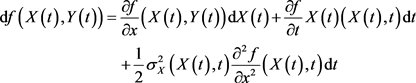 (12)
(12)
Stochastic Calculus. Let 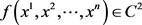 and
and  and
and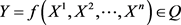 . We denote by Q the totality of quasimartingales.
Definition 2.4.1. [36] For , we say that X and Y are equivalent and write
  if, with probability one,
 for every
 .
.
The equivalence class containing X is denoted by dX and is called the stochastic differential of X. As known, by definition,

is the process .
.
Let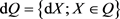 ,
,  and
and . We introduce the following operations in dQ [36].
(1) Addition:  for
for .
.
(2) Product: ![]() for
for ![]() where
where ![]() and
and ![]() are the martingale parts of X and i respectively.
are the martingale parts of X and i respectively.
(3) B-multiplication: If ![]() and
and![]() , then
, then
![]()
is defined as an element in Q. Hence ![]() is defined from
is defined from ![]() and dX. We define an element
and dX. We define an element ![]() of dQ by
of dQ by![]() .
.
Theorem 2.5. [36] The space dQ with the operations (1), (2) and (3) is a commutative algebra over B, i.e., a commutative ring with the operations (1) and (2) satisfying the relations
(a)![]() ,
,
(b)![]() ,
,
(c)![]() ,
,
(d)![]() ,
,
for ![]() and
and![]() . We also have that
. We also have that![]() ,
, ![]() and
and![]() .
.
If ![]() and
and![]() , then
, then ![]() and
and
![]() (13)
(13)
where ![]() and
and ![]() are elements in B defined by
are elements in B defined by ![]() and
and![]() , respectively. If
, respectively. If ![]() and
and![]() ,
, ![]() then
then ![]() is a d-dimensional Wiener process. Such a system of martingales
is a d-dimensional Wiener process. Such a system of martingales ![]() is called a d-dimensional Wiener martingale.
is called a d-dimensional Wiener martingale.
(4) Symmetric Q-Multiplication
![]() or
or ![]() and
and ![]()
Theorem 2.6. [35] [36] The space dQ with the operations (1), (2), (3) and (4) is a commutative algebra over Q; we have for![]() ,
,
![]()
![]()
![]()
![]()
where ![]() denotes Stratonovich product.
denotes Stratonovich product.
Theorem 2.7. If ![]() and
and![]() , then for
, then for ![]() we have
we have
![]() (14)
(14)
The stochastic integral ![]() is called the Stratonovich integral or the Fisk integral or sometimes the Fisk-Stratonovich symmetric integral. Indeed, we have the following theorem:
is called the Stratonovich integral or the Fisk integral or sometimes the Fisk-Stratonovich symmetric integral. Indeed, we have the following theorem:
Theorem 2.8. [36] For every X and Y in Q,
![]() (15)
(15)
where ![]() denotes a partition
denotes a partition ![]() and
and
![]() ,
,![]() .
.
Skorokhod Integral. The Skorohod integral is an extension of the Itô integral to non-adapted processes and is the adjoint of the Malliavin derivative, which is fundamentals to the stochastic calculus of variations [41] [42].
Definition 2.8.1. [41] Assume that
![]() (16)
(16)
Then we define the Skorohod integral of ![]() denoted by
denoted by
![]()
by
![]() (17)
(17)
where ![]() represents the Kronecker product.
represents the Kronecker product.
Wick Product. The Wick product was introduced in Wick (1950) as a tool to renormalize certaint infinite quantities in quantum field theory. In stochastic analysis the Wick product was first introduced by Hida and Ikeda (1995). The Wick product is important in the study of stochastic differential equations. In general, one can say that the use of this product corresponds to and extends naturally—the use of the Itô integrals. The Wick product can be defined in the following way:
Definition 2.8.2. The Wick product ![]() of to elements
of to elements
![]() (18)
(18)
with ![]() is defined by
is defined by
![]() (19)
(19)
In the ![]() cas the basis independence of the Wick product can be seen from the following formulation of Wick multiplication in terms of multiple Itô integrals.
cas the basis independence of the Wick product can be seen from the following formulation of Wick multiplication in terms of multiple Itô integrals.
Proposition 2.8.1. Let![]() . Assume that
. Assume that ![]() have the following representation in terms of multiple Itô integrals:
have the following representation in terms of multiple Itô integrals:
![]() (20)
(20)
Suppose![]() . Then
. Then
![]() (21)
(21)
For the relation between the Wick multiplication and The Itô-Skorohod Integration we put ![]() for simplicity. One of the most stricking features of the Wick product is its relation to Itô-Skorokhod Integration. In short, this relation can be expressed as
for simplicity. One of the most stricking features of the Wick product is its relation to Itô-Skorokhod Integration. In short, this relation can be expressed as
![]() (22)
(22)
Here the left hand side denotes the Skorokhod integral of the Stochastic process ![]() (which coincides with the Itô integral if
(which coincides with the Itô integral if ![]() is adapted), while the right hand side is to be interpreted as an
is adapted), while the right hand side is to be interpreted as an ![]() -valued (Pettis) integral. The relation 22 explains why the Wick product is so natural and importnat in stochastic calculus.
-valued (Pettis) integral. The relation 22 explains why the Wick product is so natural and importnat in stochastic calculus.
3. Stochastic Differential Equations Models
The objective of this section presents in short the two main types of stochastic differential equation models. The theory of stochastic differential equation is very vaste and well known by Engineers and other scientists but less known and understood among economists. For further reading the reader can see [36] [43] - [48].
Example 1: Stochastic Differential Equation Model. Let ![]() be a diffusion in n dimensions described by the multidimensional stochastic differential equation
be a diffusion in n dimensions described by the multidimensional stochastic differential equation
![]() (23)
(23)
where ![]() is
is ![]() matrix valued function,
matrix valued function, ![]() is d-dimensional Brownian motion and and X and
is d-dimensional Brownian motion and and X and ![]() are n-dimensional vector valued functions. The vector
are n-dimensional vector valued functions. The vector ![]() and the matrix
and the matrix ![]() are the coefficients of the stochastic differential equation.
are the coefficients of the stochastic differential equation.
Theorem 3.1. [34] (Uniqueness and Existence of Solution) If the coefficients are locally Lipschitz in X with a constant independent of t; that is, for every N, there is a constant K depending only on T and N such that for all ![]() and all
and all![]() ,
,
![]() (24)
(24)
for any given ![]() the strong solution to stochastic differentional Equation (27) is unique. If in addition to condition 24 the linear growth condition holds
the strong solution to stochastic differentional Equation (27) is unique. If in addition to condition 24 the linear growth condition holds
![]() (25)
(25)
![]() is independent of B, and
is independent of B, and![]() , then the strong solution exists and is unique on
, then the strong solution exists and is unique on![]() , moreover,
, moreover,
![]()
where the constant C depends only on K and T.
The following theorem gives the solution of stochastic differential equations as Markov processes.
Theorem 3.2. [34] (The solution of SDEs as Markov processes) If equation 27 satisfies the conditions of the existence and uniqueness theorem 3.1, the solution ![]() of the equation for arbitrary initial values is a Markov process on the interval
of the equation for arbitrary initial values is a Markov process on the interval ![]() whose initial probability distribution at the instant to is the distribution of C and whose transition probabilities are given by
whose initial probability distribution at the instant to is the distribution of C and whose transition probabilities are given by
![]() (26)
(26)
where ![]() is the solution of equation.
is the solution of equation.
Theorem 3.3 [34] (The solution of SDEs as Diffusion processes) The condition of the existence and uniqueness theorem 3.1 are satisfied for the SDE
![]() (27)
(27)
where![]() ,
, ![]() ,
, ![]() and
and ![]() is a
is a ![]() matrix. If in addition, the functions
matrix. If in addition, the functions ![]() and
and ![]() are continuous with respect to t, the solution
are continuous with respect to t, the solution ![]() is a d-dimensional diffusion process on
is a d-dimensional diffusion process on ![]() with drift vector and diffusion matrix
with drift vector and diffusion matrix![]() . In particular, the solution of an autonomous SDE is always a homogeneous diffusion process on
. In particular, the solution of an autonomous SDE is always a homogeneous diffusion process on![]() .
.
Example 2: Differential Equation with Markovian Switching Model. For economists, the economic phenomena can be governed by uncertainties and cycles. This model was developped by [49] as hybrid models. Consider the Stochastic Differential Equation with Markovian Switching of the form
![]() (28)
(28)
Here the state vector has two components: ![]() and
and![]() . The first one is normally referred to as the state while the second one is regarded as the mode. In its operation, the system will switch from one mode to another in random way, and the switching among the modes governed by the Markov chain
. The first one is normally referred to as the state while the second one is regarded as the mode. In its operation, the system will switch from one mode to another in random way, and the switching among the modes governed by the Markov chain![]() .
.
Example 3: Differential with Respect to Fractional Brownian Motion Model. Let ![]() be a m-dimensional fractional Brownian motion of Hurst parameter
be a m-dimensional fractional Brownian motion of Hurst parameter![]() . This means that the components of B are independent fractional Brownian motions with the same Hurst parameter H. For further reading see [46] [50] [51].
. This means that the components of B are independent fractional Brownian motions with the same Hurst parameter H. For further reading see [46] [50] [51].
Consider the equation on ![]()
![]() (29)
(29)
where ![]() is an m-dimensional random variable.
is an m-dimensional random variable.
Assumption 3.3.1. Let us introduce the following assumptions on the coefficients:
A1. ![]() is differentiable in x, and there exists some constants
is differentiable in x, and there exists some constants ![]() and for every
and for every ![]() there exist
there exist ![]() such that the following properties hold:
such that the following properties hold:
![]()
![]()
![]()
A2. The coefficient ![]() satisfies for every
satisfies for every ![]()
![]()
![]()
where![]() ), with
), with ![]() and for some constant
and for some constant![]() .
.
Consider the stochastic differential equation with respect to fBm (29) on ![]() where the process B is a d-dimensional fBm with Hurst parameter
where the process B is a d-dimensional fBm with Hurst parameter ![]() and
and ![]() is an m-dimensional random variable.
is an m-dimensional random variable.
Suppose that the coefficients ![]() are measurable functions satisfying conditions A1 and A2, where the constants
are measurable functions satisfying conditions A1 and A2, where the constants ![]() and
and ![]() may depend on
may depend on![]() , and
, and![]() ,
,![]() . Fix
. Fix ![]() such that
such that ![]() a uniue continuous solution such that
a uniue continuous solution such that ![]() for all
for all![]() . Moreover the solution is Holder continuous of order
. Moreover the solution is Holder continuous of order![]() .
.
Example 4: Differential Equation with Jumps Models. In real world, some phenomena or economic policy decisions are governed under uncertainty with jumps. Therefore, stochastic differential equation with jumps modeling can be considered as a usefull econometric approach [32]. Consider a one-dimensional SDE, d = 1, in the form
![]() (30)
(30)
for![]() , with
, with![]() , and
, and ![]() an
an ![]() -adapted one-dimensional Wiener process. We assume an an
-adapted one-dimensional Wiener process. We assume an an ![]() -adapted Poisson measure
-adapted Poisson measure ![]() with mark space
with mark space ![]() and with intensity measure
and with intensity measure![]() , where
, where ![]() is a given probability distribution function for the realizations of the marks. Consider a one-dimensional SDE with Jumps (30) in integral form, is of the form
is a given probability distribution function for the realizations of the marks. Consider a one-dimensional SDE with Jumps (30) in integral form, is of the form
![]() (31)
(31)
Example 5: Partial Differential Equation Models. Stochastic Partial Differential Equation Models are used as power tools of mathematical modeling in many areas [52] [53] [54].
Consider the Itô Stochastic Partial Differential Equation of the form as mentioned in [27]
![]() (32)
(32)
for![]() , where
, where![]() , is an infinite dimensional Wiener process of the form
, is an infinite dimensional Wiener process of the form
![]() (33)
(33)
with independent scalar Wiener processes![]() ,
, ![]() and. Note that
and. Note that ![]() (Laplacian with Dirichlet boundary conditions) and
(Laplacian with Dirichlet boundary conditions) and ![]() in one spatial dimension has sample paths which are only
in one spatial dimension has sample paths which are only ![]() -Hölder continuous. Here the family
-Hölder continuous. Here the family![]() ,
, ![]() , is an orthonormal basis in,
, is an orthonormal basis in,![]() .
.
Assumption 3.3.2. [27] (1) Linear operator A. Let ![]() be a finite or countable set. In addition, let
be a finite or countable set. In addition, let ![]() be a family of real numbers with
be a family of real numbers with ![]() and let
and let ![]() be an orthonormal basis of H. The linear operator
be an orthonormal basis of H. The linear operator ![]() is given by
is given by ![]() for all
for all ![]() with
with![]() . (2) Drift term F. Let
. (2) Drift term F. Let ![]() be real numbers with
be real numbers with ![]() and let
and let ![]() be a globally Lipschitz continuous mapping. (3) Diffusion term B. Let
be a globally Lipschitz continuous mapping. (3) Diffusion term B. Let ![]() be real numbers with
be real numbers with ![]() and let
and let ![]() be a globally Lipschitz continuous mapping. (4) Initial value
be a globally Lipschitz continuous mapping. (4) Initial value![]() : Let
: Let ![]() and
and ![]() be real numbers and let
be real numbers and let ![]() be an
be an ![]() -measurable mapping with
-measurable mapping with![]() .
.
The literature contains many existence and uniqueness theorems for mild solutions of SPDEs. Theorem below provides an existence, uniqueness, and regularity result for solutions of SPDEs with globally Lipschitz continuous coefficients in the Equation (32).
Theorem 3.4. [27] Let Assumptions 3.3.2 (1)-(4) be fulfilled. Then there exists a unique of the Equation (32) that is predictable stochastic process
![]() satisfying
satisfying ![]() and
and
![]() (34)
(34)
![]() for all
for all![]() . In addition,
. In addition,![]() .
.
4. Numerical Methods for Stochastic Differential Equations
In this section we give a brief review some numerical methods used in the stochastic analysis that can be usefull for economists and social scientists. These main books can help econometricians and economists to improve and understand the numerical methods for stochastic analysis [27] [45] [55] - [61]. The numerical methods for stochastic ordinary differential equations can be summarized as follows.
The Euler-Maruyama Scheme. We consider a scalar Itô stochastic ordinary differential equation (SODE) [27]
![]() (35)
(35)
with a standard scalar Wiener process![]() . The SODE (35) is in fact a symbolic representation for the stochastic integral equation
. The SODE (35) is in fact a symbolic representation for the stochastic integral equation
![]() (36)
(36)
The simplest numerical scheme for the SODE (35) is the Euler-Maruyama Scheme given by
![]() (37)
(37)
where one usually writes
![]()
for ![]() and where
and where ![]() with
with ![]() is an arbitrary partition of
is an arbitrary partition of![]() .
.
The Milstein Scheme [27]. The another useful numerical scheme for the SODE (35) is the Milstein Scheme given by
![]() (38)
(38)
Numerical Methods for Stochastic Differential Equations with Jumps. The Euler scheme for SDE with jumps (30), is given by the algorithm [32] [62] [63],
![]()
![]() (39)
(39)
for ![]() with initial value
with initial value![]() . Here
. Here ![]() is the length of the time interval
is the length of the time interval ![]() and
and ![]() is the nth Gaussian
is the nth Gaussian ![]() distributed increment of the Wiener process W,
distributed increment of the Wiener process W, ![]() ,
, ![]() represents the total number of jumps of Poisson random measure up to time t, which is Poisson distributed with mean
represents the total number of jumps of Poisson random measure up to time t, which is Poisson distributed with mean![]() .
.
In the multidimensional case with mark-indepedent jump size we obtain the kth component of the Euler scheme
![]() (40)
(40)
Methods for Stochastic Partial Differential Equations. This material is from [64]
![]() (41)
(41)
Methods for SPDE with Multiplicative Noise. Two representative numerical schemes used in the literature for the Stochastic Partial Differential Equation (32) are the linear-implicit Euler and the linear-implicit Crank-Nicolson schemes [27].
The Euler scheme
![]() (42)
(42)
The Crank-Nicolson scheme
![]() (43)
(43)
for ![]() and
and![]() . Here it is necessary to assume that
. Here it is necessary to assume that ![]() for all
for all ![]() in Assumptions 2 in order to ensure that
in Assumptions 2 in order to ensure that ![]() is inversible for every
is inversible for every![]() .
.
Convergence of SPDE with Multiplicative Noise. The convergence of the exponential Euler scheme will proved under the following assumptions.
Assumption 4.0.1. (A5) (Linear operator A). there exist sequences of real eigenvalues ![]() and orthonormal eigenfunctions
and orthonormal eigenfunctions ![]() of
of ![]() such that the linear operator
such that the linear operator ![]() is given by
is given by
![]()
for all ![]() with
with![]() .
.
(A6) (nonlinearity of F). The nonlinearity ![]() is two times continuously Fréchet differentiable and its derivatives satisfy the following conditions
is two times continuously Fréchet differentiable and its derivatives satisfy the following conditions
![]()
![]()
for all![]() ,
, ![]() , and
, and![]() , and
, and
![]()
for all![]() , where
, where ![]() is a positive constant.
is a positive constant.
Let Q be a nonnegative definite symmetric trace-class operator on a separable Hilbert space K, ![]() be an ONB in K diagonalizing Q, and let the correspoing eigenvalues be
be an ONB in K diagonalizing Q, and let the correspoing eigenvalues be![]() . Let
. Let![]() ,
, ![]() , be a sequence of independent Brownian motion defined on filtered probability space
, be a sequence of independent Brownian motion defined on filtered probability space![]() . The process
. The process ![]() is called a Q-Wiener process in K.
is called a Q-Wiener process in K.
(A7) (Cylindrical Q-Wiener process![]() ) There exist a sequence
) There exist a sequence ![]() of positive real numbers and a real number
of positive real numbers and a real number ![]() such that
such that
![]()
and pairwise independent scalar ![]() -adapted Wiener process
-adapted Wiener process ![]() for
for![]() . The cylindrical Q-Wiener process
. The cylindrical Q-Wiener process ![]() is given formally by
is given formally by
![]() (44)
(44)
(A8) (Initial value). The random variable ![]() satisfies
satisfies![]() , where
, where ![]() is given in A7.
is given in A7.
The convergence theorem for SPDE model 32
Theorem 4.1. (Convergence Theorem [27] ) Suppose that Assumptions 3 (A5)-(A8) are satisfied. Then there is a constant ![]() such that
such that
![]() (45)
(45)
holds for all![]() , where
, where ![]() is the solution of SPDE 32,
is the solution of SPDE 32, ![]() is the numerical solution given by 42,
is the numerical solution given by 42, ![]() for
for![]() , and
, and ![]() is the constant given in Assumption A8.
is the constant given in Assumption A8.
5. Application to Stochastic Volatility Estimation
Continuous-time models are central to financial econometrics, and mathematical finance. Here we estimate the Unobserved Stochastic Volatility of Inflation Rate. The literature on discrete-time models and that on continuous-time models were developed independently, but it is possible to establish connections between the two approaches [22] [23] [65] [66] [67] [68] [69].
In time series analysis, autoregressive integrated moving average (ARIMA) models have found extensive use since the publications of Box and Jenkins (1976) [25] [70] [71].
Maximum likelihood methods are widely used for estimating stochastic volatility [18].
To facilitate our discussion we will specialize the general continuous time model with zero drift, i.e.
![]() (46)
(46)
![]() (47)
(47)
where the stochastic processes![]() , and
, and ![]() are
are ![]() adapted. Here
adapted. Here ![]() is a stationary process with nonnegative values and is called the stochastic volatility. The
is a stationary process with nonnegative values and is called the stochastic volatility. The ![]() is the speed of adjustment of y to its long-run mean,
is the speed of adjustment of y to its long-run mean, ![]() , and
, and ![]() is a positive scalar. And also
is a positive scalar. And also ![]() is a standard Wiener process.
is a standard Wiener process.
One should note that the constant elasticity variance process (CEV) in 47 implied an autoregressive model in discrete time for![]() , namely:
, namely:
![]() (48)
(48)
![]() (49)
(49)
After some algebraical manipulations such as![]() ,
, ![]() and
and ![]() and
and![]() ,
, ![]() , we have this hybrid model that has the autoregssive model and the generalized autoregressive condintionally heteroscedastic models, i.e. the AR (1)-GARCH (1, 1) Model with the mean equation [13] [19] [25] [70] [72] [73],
, we have this hybrid model that has the autoregssive model and the generalized autoregressive condintionally heteroscedastic models, i.e. the AR (1)-GARCH (1, 1) Model with the mean equation [13] [19] [25] [70] [72] [73],
![]() (50)
(50)
where![]() ,
, ![]() with
with ![]() following a t-Student distribution and the variance equation that can be presented as follows
following a t-Student distribution and the variance equation that can be presented as follows
![]() (51)
(51)
where ![]() is a vector of two standard dimensional Brownian motions that are independent with zero mean and unit variance, and are defined on probability space
is a vector of two standard dimensional Brownian motions that are independent with zero mean and unit variance, and are defined on probability space![]() .
.
In time series analysis, a process ![]() is called a GARCH(p,q) process if its first two conditional moments exist and satisfy [13]
is called a GARCH(p,q) process if its first two conditional moments exist and satisfy [13]
(1)![]() ,
,![]() .
.
(2) There exist constants![]() ,
, ![]() and
and ![]() such that
such that
![]()
Theorem 5.1. ( [13] Strict stationarity of the strong GARCH (1, 1) process) if
![]()
then the infinite sum
![]()
converges almost surely (a.s.) and the process (![]() ) defined by
) defined by ![]() is the unique strictly stationary solution of the model
is the unique strictly stationary solution of the model![]() . This solution is nonanticipative and ergodic. If
. This solution is nonanticipative and ergodic. If ![]() and
and![]() , there exists no strictly stationary solution.
, there exists no strictly stationary solution.
Another important theorem for our analysis is the secon-order stationarity of the GARCH (1, 1) process.
Theorem 5.2. Let![]() . If
. If![]() , a nonanticipative and second-order stationary solution to the GARCH(1,1) model does not exist. If
, a nonanticipative and second-order stationary solution to the GARCH(1,1) model does not exist. If![]() , the process (
, the process (![]() ) defined by (2.13) is second-order stationary. More precisely (
) defined by (2.13) is second-order stationary. More precisely (![]() ) is a weak, white noise. Moreover, there exists no other second-order stationary and nonanticipative solution.
) is a weak, white noise. Moreover, there exists no other second-order stationary and nonanticipative solution.
To estimate the parameters of these models we use the maximum likelihood method. The maximum likelihood method provides the best estimators and efficient estimators [13] [73] - [78]. The density f of the strong write noise is assumed known. This assumption is obviously very strong. Conditionally on the ![]() -field
-field ![]() generated by
generated by![]() , the variable
, the variable ![]() has the density
has the density![]() . It follows that given the observations
. It follows that given the observations![]() , and the initial values
, and the initial values![]() ,
, ![]() the conditional likelihood is defined by
the conditional likelihood is defined by
![]()
where the ![]() are recursively, defined for
are recursively, defined for![]() , by
, by
![]()
For the student’s t-distribution, the log-likelihood contributions are of the form
![]()
where the degree of freedom ![]() controls the tail behavior and log denotes the natural logarithm, that is, loge where
controls the tail behavior and log denotes the natural logarithm, that is, loge where![]() . The t-distribution approaches the normal as
. The t-distribution approaches the normal as ![]() and
and ![]() denotes the Gamma function.
denotes the Gamma function.
A maximum likelihood estimator (MLE) is obtained by maximizing the likelihood on a compact subset ![]() of the parameter space [13] [79] [80] [81] that is,
of the parameter space [13] [79] [80] [81] that is,
![]() (52)
(52)
To select a fitted model, the Akaike (1973) information criterion (AIC), Schowrz (1978) information (SIC), the mean squared error criterion (SIC), Hannan-Quinn information criterion (HQC) are usually used, that is,
![]()
![]()
where ![]() refers to the number of estimated model parameters.
refers to the number of estimated model parameters.
![]()
![]()
where ![]() is the log-likelihood, k is the number of parameters, and n is the number of observations. Among a finite set of models; the model with the lowest criteria is preferred.
is the log-likelihood, k is the number of parameters, and n is the number of observations. Among a finite set of models; the model with the lowest criteria is preferred.
6. Empirical Results
In this study we modelize the stochastic volatility of inflation rate observed by the Central Bank of Congo for the period from January 2004 to June 2018. We get the inflation rate by transforming the consumer price index (CPI) index by using log-difference transformation, that is,![]() . The operations of taking logarithms and differencing are standard time series tools for coering a data set into looking stationary (Resnick, 2007); therefore our variable is stationary. The inflation rate measures how fast prices are rising [21] [82]. For the period under analysis Table 1 shows that the mean, the maximum, and minimum inflation rates are 1.3, 11.4, −7.5 percentages respectively. (ii) With the Jarque-Bera statistic, 346.8773, it indicates that the inflation rate does not follow the normal distribution. It is well known that the fundamental task in many statistical analyses is to characterize the location and variability of a data set. A further characterization of the data includes skewness and kurtosis. The Skewness statistics is a measure of symmetry, or more precisely, the lack of symmetry. A distribution, or data set, is symmetric if it looks the same to the left and right of the center point. The Skewness of 1.52 indicates the moderate level.
. The operations of taking logarithms and differencing are standard time series tools for coering a data set into looking stationary (Resnick, 2007); therefore our variable is stationary. The inflation rate measures how fast prices are rising [21] [82]. For the period under analysis Table 1 shows that the mean, the maximum, and minimum inflation rates are 1.3, 11.4, −7.5 percentages respectively. (ii) With the Jarque-Bera statistic, 346.8773, it indicates that the inflation rate does not follow the normal distribution. It is well known that the fundamental task in many statistical analyses is to characterize the location and variability of a data set. A further characterization of the data includes skewness and kurtosis. The Skewness statistics is a measure of symmetry, or more precisely, the lack of symmetry. A distribution, or data set, is symmetric if it looks the same to the left and right of the center point. The Skewness of 1.52 indicates the moderate level.
In statistics, the Kurtosis is a measure of whether the data are heavy-tailed or light-tailed relative to a normal distribution. That is, data sets with high kurtosis tend to have heavy tails, or outliers. Data sets with low kurtosis tend to have light tails, or lack of outliers. Kurtosis statistics of the inflation rate 9.23 more large than 3, and Jarque-Bera statistics indicate that inflation rate does not follow the normal distribution. With high kurtosis statistic, 9.2287, there is an indication of inflation volatility.
We use a Student statistic test of statistical significance and find that parameters estimations are all statistically significant. Results confirm that the past volatilities affect the current volatility of inflation rate. Thus, we the dynmical behavior of volatility. We restrict the constant term to a function of the GARCH parameters and the unconditional variance:
![]()
where ![]() is the unconditional variance of the residuals, that is,
is the unconditional variance of the residuals, that is,![]() .
.
Table 2 raises tree isues. First, in the mean equation, the coefficient ![]() measuring the persistence of inflation rate is high. This means that the monthly last inflation contributes to current rate by 66 percents. Secondly, the stochastic
measuring the persistence of inflation rate is high. This means that the monthly last inflation contributes to current rate by 66 percents. Secondly, the stochastic
volatility persistence of CPI-inflation rate is very high level, ![]() , this means that the past volatility information contributes to current volatility of inflation rate at 100 percents. Therefore the purchasing power of congolese householders is also volatile.
, this means that the past volatility information contributes to current volatility of inflation rate at 100 percents. Therefore the purchasing power of congolese householders is also volatile.
The postestmation tests of Ljung Box (1978), Q-Stat = 3.0639, and ARCH test, 0.0171, show that there are any remaining ARCH effects in the residuals.
7. Concluding Remarks
Since the Itô’s works, the stochastic integrals and stochastic differential equations attract the attention of many researchers in the fields of mathematical modelling. In this paper, we emphasize on the application of stochastic integrals and differential equations in the economics and finance. Comparing to discrete models, the stochastic continuous-time models have many advantages because they take into account the uncertainty. The limit of this approach is the complexity of stochastic calculus and stochastic numerical methods. As mentioned by scientists (see Wiener, Einstein, Itô) the uncertainties are anywhere and anytime; therefore the stochastic integrals must be well known and understood by all scientists.