Closer Approximation to Optimize Solar Panels Performance with Cleaning Cycle: A Follow-Up

Rijan Karkee¹, Sumit Khadka²

¹Department of Physics, University of California Merced, Merced, USA.
²Department of Physics, University of Houston-Main, Houston, USA.

DOI: 10.4236/ojee.2019.84010                

Abstract

The performance of solar panels significantly degrades due to dust accumulation but cleaning too frequently will severely impact the financial benefits of the installation of solar panels. This paper assumes a realistic linear model for accumulation of dust on the solar panels and the resulting hourly average of absolute loss of efficiency in solar panels. This model accurately depicts the fact that energy production by solar panels occurs during sunshine hours only and also accounts for the degradation in the efficiency of solar panels due to dust accumulation throughout the entire day. Based on this, the optimal number of days for maximum financial profit and the critical number of days (above which there is no profit in installing solar panels) have been estimated. Furthermore, we have suggested a formalism to help estimate the finances for self-cleaning technology for PV system and also for calculating the minimum payback period for installing solar panels with the financial cost of the cleaning cycles properly considered. This research could be motivation for companies in developing self-cleaning mechanism for PV system.

Keywords

Dust Accumulation, Optimal and Critical Number of Days for Cleaning Cycles, Payback Period, Self-Cleaning System

1. Introduction

Photovoltaic (PV) system is emerging technology that can deliver electricity directly from sunlight. As concerns for clean energy rises, PV technology is becoming more popular. There have been numerous research efforts around the world to make PV technology better in terms of price, durability and efficiency. These efforts include investigating on properties of semiconductor, reducing contact losses, using solar tracker and many more. Recently, the effect of soiling has emerged as an important parameter to consider, as this significantly reduces the overall performance of PV panels.

Soiling losses are losses in efficiency of PV module due to deposition of dust, dirt, snow thereby covering the active area of solar panels. Zaki Ahmad et al. [1] in 2014 categorized the dust that affects the soiling in PV panel into classes such as red soil, cement, ash, carbon, limestone, sand etc. Many researchers have studied the effect of dust on solar panels [2] [3] [4] [5] and found degradation does occur to some degree in solar efficiency due to dust deposition. The quantity and rate of dust accumulation depend on tilt of the solar panels, wind speed, the roughness of the surface, and environment conditions [6]. Since dust accumulation directly affects the performance of the PV panels, it is strongly advised to clean the PV panel frequently for better performance of solar devices. Author in [7] describes the most commonly used cleaning techniques which include cleaning by rainfall, manual cleaning and mobile cleaners. Kimber et al. [8] have stated that at least 20 mm rainfall is needed to clean PV modules (annual rainfall below 20 mm actually resulted in decrease in the efficiency). Unfortunately, rainfalls are not common and occur periodically in a year for most places. However, there are several cleaning technologies introduced in the market which ranges from simple manual cleaning to automatic cleaning system [9].

Sanaz Ghazi et al. [10] have investigated the pattern of dust distribution in different parts of the world and introduced a parameter, α, the daily average loss in solar efficiency varies from place to place around the world and it is an important parameter considered to optimize the economics from solar panel. There are few other examples [11] [12] [13] where authors have experimentally calculated the daily average loss in efficiencies in area such as California, Chile, Qatar.

While cleaning will definitely help to improve the performance of PV, it certainly comes up with some financial costs. Abu-Naser [14] calculated the optimal number of days for cleaning cycles that would result in the least financial cost of overall installation of PV panels (or arrays as well) and found out that the optimal number of days for cleaning cycles is given as:

$N^{opt}=\sqrt{\frac{2P}{is\alpha \beta }}$, #(1)

where $\alpha$ is the average daily degradation in the solar conversion efficiency, i is the capacity of the installed PV system, $\beta$ is the price of kWh, s is the average sun hours per day. There are basically two things that we would want to upgrade to previous model which were not taken into consideration in the model.

Here we follow a similar methodology as presented in [14] with major modifications and added interpretation. We account for the fact that the financial gain by using solar panels is achieved during the sunshine hours only but the degradation due to soiling does continue at the same rate outside the sunshine hours as well.

Firstly, the author [14] has assumed degradation in efficiency as constant throughout the day and has used the value that is to be observed at the end of day. But degradation happens continuously throughout the day. Secondly, the solar modules can only generate electricity (most efficiently) during sunshine hours and we should account the degradation in efficiency due to soiling in that period. In this paper, we tackle the first part by taking the average loss in efficiency from beginning of sunshine hour to end of sunshine hour which validates the linear model for degradation of efficiency with exact losses in an hourly basis. For the second part, we assumed hourly loss in degradation and used it to find losses in performance efficiency up to sunshine hours. Since the degradation can also happen after sunshine hours, we’ve incorporated this loss after sunshine hour in the following day’s calculation. In the following section, we follow up methodology introduced in [14] to include better approximation as discussed here and present the optimal frequency of cleaning and other relevant calculation.

2. Formulation

This section discusses about implementing the modifications and methodology as stated in previous section. For a solar panel of capacity i, efficiency ${\eta }_0$, with s sunshine hours per day, $\beta$ the price of unit electricity in kWh (obtained from sources other than solar) than the financial savings due to installing solar panel is given by,

$S=is\beta$, #(2)

where $i={\eta }_0{P}_{in}$ ; $P_{in}$ being the incident solar radiation.

The dust accumulation will result in decrease in the efficiency of the solar panel, say ${\eta }_1$, then the power output of the solar panel would be ${P^{\prime }}_{out}={\eta }_1{P}_{in}$ and the financial savings at this condition is:

$S_1={\eta }_1{P}_{in}s\beta$. #(3)

This would imply that the financial loss due to dust accumulation when the efficiency of the solar panel drops from ${\eta }_0$ to ${\eta }_1$ is

$Loss=\left({\eta }_0-{\eta }_1\right)\frac{i}{{\eta }_0}s\beta$. #(4)

We have assumed a simple yet a realistic scenario where the solar panel is in operation only during the sunshine hours and assumes it has constant efficiency ${\eta }_0$ when there is no dust accumulation.

If we assume that the dust accumulation is uniform and degradation rate in efficiency is constant per day, we can come up with following scenario for the efficiencies of the solar panels as presented in Figure 1.

The dust accumulation is considered linear, so the financial loss at the end of first s sunshine hours is given as:

$Los{s}_{1s}=\left({\eta }_0-{\eta }_{01}^{av}\right)\frac{i}{{\eta }_0}s\beta$, #(5)

where ${\eta }_{01}^{av}=\left({\eta }_0+{\eta }_1\right)/2$.

Figure 1. Simple linear model for degradation of efficiency due to dust accumulation. The shaded (in blue) parts indicate the night period where solar panel can’t produce electricity. ${\eta }_{i\left(i=0,1,2,3,\cdots \right)}$ are the efficiencies at the end of certain hour “s”.

This is also the financial loss for the entire first day since during night no savings is acquired due to installation of solar panels (no sunshine). There is still dust accumulation during the night though and the efficiency drops to ${\eta }_2$ at the start of the second day.

We will introduce a term ${\alpha }^{\prime }$ which is defined as hourly average of absolute loss of efficiency in solar panels. It is realistic to assume an average hourly loss in solar conversion efficiency as it can most easily be related to the rate of dust accumulation in the solar panels. This would imply, ${\eta }_s={\eta }_0-{\alpha }^{\prime }s$ giving exact efficiency after s hours. Similarly, if we want to define absolute loss in terms of day, lets introduce f as daily average of absolute loss in efficiency so that efficiency after N days will be ${\eta }_N={\eta }_0-fN$ as illustrated in the schematic below.

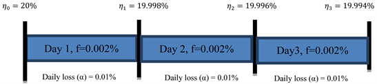
To better understand this in terms of α which is defined as average daily loss in solar efficiency (as used in [14] model), let’s suppose average daily loss in solar conversion efficiency α = 0.01% and also suppose panel is 20% efficient under clean condition. Then from Equation (2) and Equation (3) of [14], the efficiency after 1^st day reduces to 19.998%. So, in this case, f will be 0.002%. With this value of f, we can keep track of exact value of efficiency after every N days.

So, defining average of absolute loss in efficiency preserves the fact of average of daily loss in solar conversion efficiency α is uniform. Similarly, the ${\alpha }^{\prime }$ in terms of f would simply be ${\alpha }^{\prime }=f/24$. The relation between f and α follow as $f=\left({\eta }_0\alpha \right)$ and the relation between α and α’ will thus be ${\alpha }^{\prime }=\left({\eta }_0\alpha \right)/24$.

If we assume a cleaning cycle of N days, the financial loss for the n^th day can be generalized by (see Appendix):

$Los{s}_n=\left[\frac{48\left(n-1\right)+s}{2}\right]\frac{i}{{\eta }_0}s\beta {\alpha }^{\prime }$. #(6)

The total financial loss per annum is

$L_1=\frac{365}{N}\underset{n=1}{\overset{N}{{\displaystyle \sum }}}\left[\frac{48\left(n-1\right)+s}{2}\right]\frac{i}{{\eta }_0}s\beta {\alpha }^{\prime }$, #(7)

$=\frac{365}{2}\frac{i}{{\eta }_0}s\beta {\alpha }^{\prime }\left[24\left(N-1\right)+s\right]$, #(8)

If P is the cost of cleaning the solar array, then the cost of cleaning per annum is

$L_2=\frac{365}{N}P$. #(9)

The total cost of installing solar array is

$L=L_1+L_2$, #(10)

$=\frac{365}{2}\frac{i}{{\eta }_0}s\beta {\alpha }^{\prime }\left[24\left(N-1\right)+s\right]+\frac{365}{N}P$. #(11)

The optimal number of days between cleaning cycles, $N^{opt}$ ; which is also the minimum value of N, calculated by differentiating Equation with respect to N and equating it to zero is

$N^{opt}=\sqrt{\frac{{\eta }_{0}P}{12is{\alpha }^{\prime }\beta }}$. #(12)

If we convert hourly loss in efficiency due to soiling into daily loss in efficiency (i.e. ${\alpha }^{\prime }$ to $\alpha$ by setting ${\alpha }^{\prime }=\left({\eta }_0\alpha \right)/24$ we obtain similar equation in terms of α presented in Equation (1) i.e.

$N^{opt}=\sqrt{\frac{2P}{is\alpha \beta }}$. #(13)

Similarly, following the same procedures, if we assume ${\gamma }^{\prime }$ and ${\gamma }^{″}$ to be average of absolute loss in efficiency during sunshine hour s and night hours (24 - s) respectively. We assume different rates of soiling during day and night because human activities might induce different soiling rates. For such approximation, if we follow similar procedures as in Appendix 1 and Appendix 2, we get

$N^{opt}=\sqrt{\frac{2{\eta }_{0}P}{is\beta \left[{\gamma }^{\prime }s+{\gamma }^{″}\left(24-s\right)\right]}}$. #(14)

Equation (14) converges to Equation (13) if rates of degradation are same ( ${\gamma }^{\prime }={\gamma }^{″}$ ) throughout day. Equation (14) is a more general form and accounts for optimal cleaning days if the degradation rates vary during the sunshine and outside it.

3. Discussion

In this section, we follow through the different parameters in the formulation section and compare the results with existing models as well as interpret and extend the formalism to yield further outcomes. This includes computing total difference in financial loss per year with this model and the existing model in [14], aspects of self-cleaning mechanism, calculation of payback period, introducing sensible and critical cleaning frequency in addition to optimal cleaning frequency.

1) Comparison of financial loss: This model and previous model yields same equation for optimal days. However, we see that this model predicts larger overall energy production per annum (accounting the soiling effects, of course) resulting in less financial loss per annum with the same cleaning frequency as compared to model presented in [14]. If we take the difference of financial loss per annum as in Equation (10) of [14] with this model represented by Equation (11), we get a difference of (say G) as:

$G=\frac{365is\alpha \beta }{2}\left(2-\frac{s}{24}\right)$. #(15)

2) Payback period and self-cleaning mechanism: Another avenue to explore is to imagine instead of manual cleaning, a self-cleaning mechanism is deployed where the cleaning machine derives power from the solar panel itself. This model implies that the calculated payback period is achieved faster than model presented in [14]. To understand it, let C be the total cost of i kilowatt solar panel including installation and X the cost of purchasing and operation of the self-cleaning machine. Then simple payback period for this model would be

$\tau =\frac{C+X}{365is\beta -los{s^{\prime }}_{\text{soiling}}-los{s}_{\text{cleaning}}}$. #(16)

If we compare this with [14], all the term in the denominator will be same except with correction term that came from our model i.e.

${\tau }^{\prime }=\frac{C+X}{365is\beta -los{s}_{\text{soiling}}-los{s}_{\text{cleaning}}}$. #(17)

Obviously, $los{s^{\prime }}_{\text{soiling}}$ is less than $los{s}_{\text{soiling}}$ by G amount (Equation (15)) giving $\tau <{\tau }^{\prime }$ indicating a simple payback period is achieved faster. It is to be noted that if self-cleaning mechanism is deployed, the $los{s}_{\text{cleaning}}$ is calculated by equivalently converting power taken to clean the device.

3) Sensible Cleaning Frequency: The other aspect that we want to introduce is Sensible Cleaning Frequency of solar module. It is defined when loss from PV module in a single day is exactly equal to cleaning cost (or equivalent energy) of the module. This is obtained by equating the financial loss at n^th day (Equation (6)) with total cost of cleaning i.e.

$\left[\frac{48\left(n-1\right)+s}{2}\right]\frac{i}{{\eta }_0}s\beta {\alpha }^{\prime }=P$. (18)

Upon solving for n, and letting $n=N_s$ for sensible cleaning frequency, we get

$N_s=1+\frac{P}{is\beta \alpha }-\frac{s}{48}$. (19)

After $N_s$ days, the loss due to soiling in a single day is greater than cost of cleaning. Therefore, it is more sensible to clean panels.

4) Critical Cleaning Frequency & Limit in Lifetime for Solar Technology: We define critical cleaning frequency as cleaning period above which there is no financial profit in installing solar panels. This is obtained by taking ratio of total cost of installing solar modules with total financial loss in T years such that the ratio is greater or equal to lifetime of solar modules. So, by following from Equations (6)-(9), the total loss in T years in terms of $\alpha$ is:

$T\frac{365}{2\times 24}i\alpha s\beta \left[24\left(N-1\right)+s\right]+T\frac{365}{N}P$. #(20)

Let C and X be cost of PV with installation and cost of cleaning machine respectively, and if we consider battery and inverter working until the solar panel lifetime (meaning no replacement and associated cost). Also, we assumed that solar panel works constantly throughout its lifetime at same constant efficiency and only loss is due to soiling. The financial gain from installation of solar panel of capacity i with average s sunshine hour and $\beta$ price per kWh in T years is $365Tis\beta$. We want to equate total production including loss with total cost for solar module system in T years as:

$T=\frac{C+X}{365is\beta -\frac{365}{48}i\alpha s\beta \left[24\left(N-1\right)+s\right]-\frac{365}{N}P}$. #(21)

which is quadratic equation in N,

$N=\frac{\left(A-\frac{sA}{24}+B\right)\mp \sqrt{{\left(A-\frac{sA}{24}+B\right)}^2-1460AP}}{2A}$. #(22)

with, $A=\frac{365is\beta \alpha }{2}$

$B=365is\beta -\frac{C+X}{T}$.

For valid solution in N, we must have

${\left(A-\frac{sA}{24}+B\right)}^2-1460AP\ge 0$. #(23)

For minimum solution,

$A-\frac{sA}{24}+B=\sqrt{1460AP}$. #(24)

$T_{\min }=\frac{C+X}{365is\beta +A-\sqrt{1460AP}-\frac{sA}{24}}$. #(25)

This $T_{\min }$ (Minimum Payback Period) carries two main information. $T_{\min }$ is directly proportional to the value of $\alpha$ meaning if we are in environment full of dust, the payback period increases. Also, if there is new solar technology, it must have at least $T_{\min }$ life period (based on Equation (25)). Another aspect that above expression provides the manufacturer company who is planning to introduce self-cleaning technology to decide how much value for X to be put to optimize the payback period.

Similarly, in the Equation (22) taking positive roots,

$N_{\text{critical}}=\frac{\left(A-\frac{sA}{24}+B\right)+\sqrt{{\left(A-\frac{sA}{24}+B\left\{\text{function}\text{of}{T}_{\text{life-cycle}}\right\}\right)}^2-1460AP}}{2A}$. (26)

Here, in the B term, if we use T as total life cycle of give solar technology (for example, in case of Silicon-based Solar cells, T = 20 years), we can get critical cleaning frequency suggesting above which there is no pay-back from installing PV system.

4. Results

We have introduced hourly average loss in efficiency because of which we were able to dive into approximation more closely. We did get better results in terms of total power production in a year or less financial loss in a year. In fact, the difference between the losses is discussed in the discussion part and is plotted (G parameter in Equation (15)) as a function of average daily loss in efficiency in Figure 2. It is to be noted that these differences become more significant when the average daily loss in efficiency (α) is greater. For example, as shown in [14] Under Section 4, with the parameters s = 5 hours, i = 1000 kW, β = 0.1, P = $250 and α = 0.002: the difference in financial loss or the G parameters is found to be $326.9. This amount is more than one-time cleaning cost (P = $250). This is really helpful in the overall finances of installing and operating a solar panel.

In discussion part, we have also derived Minimum Payback Period (T_min in Equation (25)) that emphasizes the newer solar technology to have minimum of T_min in an environment set by α parameter. This model sets limit as we have considered no other losses in efficiency except that PV performance degrades every year by 0.5% [15] [16]. This inclusion results in much higher time period. Similarly, the same equation can be tuned by setting the self-cleaning price to ensure and optimize shorter payback period. The final nomenclature we introduced in Discussion section is sensible and critical cleaning frequency. The sensible cleaning frequency relates to cleaning cost for PV system is equal to loss due to soiling whereas the critical cleaning frequency relates to no profit in installing PV system. If this value is greater or equal to 365 days and rains heavily at least once a year, there is no point to worry. However, in desert area where it does not rain and α parameter is large, one must think about cleaning at proper time. Based on α parameter found in some literature, we present optimal, sensible and critical cleaning frequencies for some places and are given in Table 1.

Table 1. Different calculated value assuming arbitrary values with parameter such as s = 5 hours, i = 1000 kW, β = $0.1, T_life = 20 years and P = $250.

Figure 2. The difference in loss per year between [14] and this model is termed as gain. Mathematically, G is obtained in Equation (15) and is plotted for different values of average daily loss in efficiency (The arbitrary values of parameters such as s = 5, i = 1000, β = 0.1 are chosen to plot this graph).

5. Conclusions

We have introduced a model with ${\alpha }^{\prime }$ which is absolute loss in conversion efficiency per hour allowing us to closely correlate the dust accumulation patterns and more accurately calculated the value for optimal, sensible and critical cleaning frequency. In addition to this, the financial savings due to installing a solar panel are achieved during sunshine hours only and this model addresses this, thereby accounting the losses more accurately. We have also calculated the payback period for installing a self-cleaning mechanism and provided a formalism to optimize its pricing for shorter payback period. Also, we have discussed how environmental factors (dust deposition) set the minimum lifetime for newer solar technologies to obtain financial benefit upon installing them. This calculation is useful to set up automatic cleaning systems to certain frequency per year depending on the value of average daily loss in efficiency at given area and to manufacture companies for deciding the cost of automatic cleaning systems (if available).

It should be noted that our model is based on linear degradation which might not be the exact case in real life. More experimental effort in determining the trend of loss due to soiling might help to accurately estimate above mentioned parameters. The only degradation in efficiency on solar panels due to soiling is assumed in this model which opens opportunity for further researches by including loss in efficiency due to other factors. Also, for payback period, more sophisticated models with discount rate and inflation rates can be incorporated better estimation.

Appendix 1.

If ${\alpha }^{\prime }$ is the hourly average of absolute loss in solar conversion efficiency loss, then the solar conversion efficiencies can be calculated as:

${\eta }_1={\eta }_0-s{\alpha }^{\prime }$,

${\eta }_2={\eta }_0-24{\alpha }^{\prime }$,

${\eta }_3={\eta }_0-\left(24+s\right){\alpha }^{\prime }$,

${\eta }_4={\eta }_0-48{\alpha }^{\prime }$,

${\eta }_5={\eta }_0-\left(48+s\right){\alpha }^{\prime }$.

and so on.

The dust accumulation is considered linear, so the financial loss at the end of first s sunshine hours is given as:

$Los{s}_{1s}=\left({\eta }_0-{\eta }_{01}^{av}\right)\frac{i}{{\eta }_0}s\beta$,

where ${\eta }_{01}^{av}=\left({\eta }_0+{\eta }_1\right)/2$.

Calculation for ${\eta }_0-{\eta }_1^{av}$ follows as:

$\begin{array}{c}{\eta }_0-{\eta }_{01}^{av}={\eta }_0-\frac{{\eta }_0+{\eta }_1}{2}\\ ={\eta }_0-\frac{{\eta }_0+{\eta }_0-s{\alpha }^{\prime }}{2}\\ =\frac{s{\alpha }^{\prime }}{2}\end{array}$,

i.e.

$Los{s}_{1s}=\frac{s{\alpha }^{\prime }}{2}\frac{i}{{\eta }_0}s\beta$.

After the s sunshine hours for the second day, $Los{s}_{2s}=\left({\eta }_0-{\eta }_{23}^{av}\right)is\beta$ with ${\eta }_{23}^{av}=\left({\eta }_2+{\eta }_3\right)/2$.

Calculation for $\left({\eta }_0-{\eta }_{23}^{av}\right)$ follows as:

$\begin{array}{c}{\eta }_0-{\eta }_{23}^{av}={\eta }_0-\frac{{\eta }_2+{\eta }_3}{2}\\ ={\eta }_0-\frac{{\eta }_0-24{\alpha }^{\prime }+{\eta }_0-\left(24+s\right){\alpha }^{\prime }}{2}\\ =\frac{\left(48+s\right){\alpha }^{\prime }}{2}\end{array}$,

i.e.

$Los{s}_{2s}=\frac{\left(48+s\right){\alpha }^{\prime }}{2}\frac{i}{{\eta }_0}s\beta$.

Similarly, $Los{s}_{3s}=\frac{\left(96+s\right){\alpha }^{\prime }}{2}is\beta$ which leads us the generalization rule Equation (6).

The total financial loss for N days, $L_0$ can be calculated by summing over the financial losses incurred during each day.

So,

$\begin{array}{c}{L}_0=\underset{n=1}{\overset{N}{{\displaystyle \sum }}}\left[\frac{48\left(n-1\right)+s}{2}\right]\frac{i}{{\eta }_0}s\beta {\alpha }^{\prime }\\ =\frac{i}{{\eta }_0}s\beta {\alpha }^{\prime }\underset{n^{\prime }=0}{\overset{N-1}{{\displaystyle \sum }}}\left[\frac{48n^{\prime }+s}{2}\right]\\ =\frac{i}{{\eta }_0}s\beta {\alpha }^{\prime }\left(\frac{s}{2}+\underset{n^{\prime }=1}{\overset{N-1}{{\displaystyle \sum }}}\left[\frac{48n^{\prime }+s}{2}\right]\right)\\ =\frac{is\beta {\alpha }^{\prime }}{2{\eta }_0}\left(s+\frac{48\left(N-1\right)N}{2}+s\left(N-1\right)\right)\\ =\frac{is\beta {\alpha }^{\prime }}{2{\eta }_0}\left(sN+24N\left(N-1\right)\right)\end{array}$.

Finally, the financial loss per annum is calculated as:

$L_1=\frac{365}{N}{L}_0$.

Appendix 2.

The optimal number of days between cleaning cycles, $N^{opt}$ is also the minimum value of N which calculated by differentiating Equation with respect to N and equating it to zero.

$\frac{\text{d}L}{\text{d}N}=0$.

Or,

$\frac{\text{d}}{\text{d}N}\left(\frac{365}{2}\frac{i}{{\eta }_0}s\beta {\alpha }^{\prime }\left[24\left(N-1\right)+s\right]+\frac{365}{N}P\right)=0$,

$\frac{365}{2}\frac{i}{{\eta }_0}s\beta {\alpha }^{\prime }\times 24-\frac{365}{N^2}P=0$,

$365\times 12\frac{i}{{\eta }_0}s\beta {\alpha }^{\prime }=\frac{365}{N^2}P$,

$N^{opt}=\sqrt{\frac{{\eta }_{0}P}{12is{\alpha }^{\prime }\beta }}$.

Conflicts of Interest

The authors declare no conflicts of interest regarding the publication of this paper.

References

[1]	Darwish, Z.A., Kazem, H.A., Sopian, K., Al-Goul, M. and Alawadhi, H. (2015) Effect of Dust Pollutant Type on Photovoltaic Performance. Renewable and Sustainable Energy Reviews, 41, 735-744. https://doi.org/10.1016/j.rser.2014.08.068
[2]	Hottel, H. and Woertz, B. (1942) Performance of Flat-Plate Solar-Heat Collectors.
[3]	Nimmo, B. and Seid, A.M.S. (1979) Effect of Dust on the Performance of Thermal and Photovoltaic Fiat Plate Collectors in Saudi Arabia: Preliminary Results. Proceedings of the 2nd Miami International Conference on Alternative Energy Sources, Miami Beach, FL.
[4]	El-Shobokshy, M.S. and Hussein, F.M. (1993) Degradation of Photovoltaic Cell Performance Due to Dust Deposition on to Its Surface. Renewable Energy, 3, 585-590. https://doi.org/10.1016/0960-1481(93)90064-N
[5]	Kaldellis, J.K. and Kapsali, M. (2011) Simulating the Dust Effect on the Energy Performance of Photovoltaic Generators Based on Experimental Measurements. Energy, 36, 5154-5161. https://doi.org/10.1016/j.energy.2011.06.018
[6]	Mani, M. and Pillai, R. (2010) Impact of Dust on Solar Photovoltaic (PV) Performance: Research Status, Challenges and Recommendations. Renewable and Sustainable Energy Reviews, 14, 3124-3131. https://doi.org/10.1016/j.rser.2010.07.065
[7]	Mohammad, R.M., Hashim, H., Chandima, G., Mohd, A.R., Mohammad, I.R. and Shahrooz, H. (2016) Power Loss due to Soiling on Solar Panel: A Review. Renewable and Sustainable Energy Reviews, 59, 1307-1316. https://doi.org/10.1016/j.rser.2016.01.044
[8]	Kimber, A., Mitchell, L., Nogradi, S. and Wenger, H. (2006) The Effect of Soiling on Large Grid-Connected Photovoltaic Systems in California and the Southwest Region of the United States. 4th IEEE World Conference on Photovoltaic Energy Conversion, Waikoloa, HI, 7-12 May 2006, 2391-2395. https://doi.org/10.1109/WCPEC.2006.279690
[9]	Deutsche Gesellshaft Für Sonnenenergie (2008) Planning and Installing Photovoltaic Systems: A Guide for Installers, Architects and Engineers. Earthscan.
[10]	Ghazi, S., Sayigh, A. and Ip, K. (2014) Dust Effect on Flat Surfaces—A Review Paper. Renew Sustain Energy Reviews, 33, 742-751. https://doi.org/10.1016/j.rser.2014.02.016
[11]	Mejia, F.A. and Kleissl, J. (2013) Soiling Losses for Solar Photovoltaic Systems in California. Solar Energy, 95, 357-363. https://doi.org/10.1016/j.solener.2013.06.028
[12]	Urrejola, E., Antonanzas, J., Ayala, P., Salgado, M., Ramrez-Sagner, G., Corts, C., Pino, A. and Escobar, R. (2016) Effect of Soiling and Sunlight Exposure on the Performance Ratio of Photovoltaic Technologies in Santiago, Chile. Energy Conversion and Management, 114, 338-347. https://doi.org/10.1016/j.enconman.2016.02.016
[13]	Javed, W., Guo, B., Wubulikasimu, Y. and Figgis, B.W. (2016) Photovoltaic Performance Degradation Due to Soiling and Characterization of the Accumulated Dust. 2016 IEEE International Conference on Power and Renewable Energy, Shanghai, 21-23 October 2016, 580-584. https://doi.org/10.1109/ICPRE.2016.7871142
[14]	Abu-Naser, M. (2017) Solar Panels Cleaning Frequency for Maximum Financial Profit. Open Journal of Energy Efficiency, 6, 80-86. https://doi.org/10.4236/ojee.2017.63006
[15]	Jordan, D.C. and Kurtz, S.R. (2012) Photovoltaic Degradation Rates—An Analytical Review. Progress in Photovoltaics: Research and Applications, 21, 12-29.
[16]	Riley, D.M., Fleming, J.E. and Gallegos, G.R. (2016) A Photovoltaic System Payback Calculator, Sandia Report, Sandia National Laboratories.