Can Really Regularized Amplitudes Be Obtained as Consistent with Their Expected Symmetry Properties?

OrimarOrimar Antônio Battistel¹, Gilson Dallabona², Marcus Vinicios Fonseca³, Luciana Ebani^2,4

¹Departamento de Física, Universidade Federal de Santa Maria, Santa Maria, Brazil.
²Departamento de Física, Universidade Federal de Lavras, Lavras, Brazil.
³Instituto Federal Farroupilha, São Vicente do Sul, Brazil.
⁴Centro Brasileiro de Pesquisas Física, Rio de Janeiro, Brazil.

DOI: 10.4236/jmp.2018.96070                

Abstract

Through a very detailed investigation involving a set of simple perturbative amplitudes we show that the answer for the question put in the title of the present work is: undoubtedly NO! We are not restricting the sentence to the amplitudes which are considered as anomalous. The referred investigation is performed by using a procedure alternative to the traditional regularization methods. In the context of such a strategy the amplitudes are not modified in intermediary steps of the calculation, like traditional regularization procedures do, and only the validity of the linearity in the integration operation is assumed in the operations made in Feynman integrals typical of the perturbative calculations. The central point of the investigation is the question related to the consistent interpretation of the amplitudes. For these purposes, in all amplitudes having power counting indicating the possibility of divergences, the relations among Green functions, Ward identities and low energy limits are analyzed, in a model having different species of massive 1/2 spin fermions coupled to spin 0 and 1 (even and odd parity) boson fields, formulated in a space-time dimension D=1+1. We show that the maintenance of the linearity in operations involving Feynman integrals excludes the possibility of an anomalous term in the Ward identity relating the axial-vector and the pseudo-scalar-vector two point functions amplitudes. In addition, we show that it is not possible the maintenance of Ward identities and low energy limits in a consistent way if the amplitudes of the perturbative calculations are quantities to be regularized, just because there is no regularization method which is capable to give acceptable results for the divergent objects present in the calculations. This conclusion includes the Dimensional Regularization method which cannot give unique results if the linearity and the symmetric integration are simultaneously required in Feynman integrals. The qualitative conclusions apply in an equally-way in other space-time dimensions having, therefore, implications in many phenomenological consequences of quantum field theories stated through perturbative solutions.

Keywords

Perturbative Calculations, Anomalies, Ward Identities, Consistency

1. Introduction

It remains no doubt about the fact that the quantum field theory represents the adequate tool for the description of relativistic interactions of fundamental particles. The quantitative results obtained, mainly in scope of quantum electrodynamics, and the qualitative accordance between experimental data and theoretical predictions, within the context of the standard model, leave no room for hesitations in to agree with the preceding sentence, specially after the recent experiments in the large hadron collider where the Higgs Bosons discovery was announced. The construction of such a formalism is a consequence of a very hard work of many peoples along many years in searching for adequate interpretations for the perturbative solutions of quantum field theory, in particular for the quantum electrodynamics. This is due to the fact that in such type of solutions the amplitudes corresponding to basic processes are plagued by infinities or divergences so that an adequate interpretation is required in order to state the physical implications. Such an interpretation is given by the renormalization which, due to this reason, has played the role of a guide for the construction of theories having physical meaning. In this conceptual point of view, the theories are required to be renormalizable to get physical significance. The renormalizability, on the other hand, is deeply related to the maintenance, in the perturbative solutions, of the symmetries implemented in the construction of the theory. At first sight it seems obvious that the solutions will reflect the symmetries of the theory. However, as it is well known, within the context of quantum field theory obvious expectations are not always materialized. We are referring to the most intriguing and subtle aspect of quantum field theory; the unavoidable violations of symmetry relations or anomalies [1] - [8] . Since the violations are unavoidable, the theories having anomalies are not renormalizable. The renormalization is only possible if different species of fermions are present at the theory so that anomalies coming from different sectors produce an exact cancellation, which is the anomaly cancellation mechanism, a fundamental ingredient of the standard model responsible for the presence of six quarks and six leptons in the theory. The anomalies eliminated in the standard model are those associated to the single (AVV) and triple (AAA) axial vector triangles. For these amplitudes it can be shown that four general expectations based on symmetries can be stated: three Ward identities and one low-energy limit. However, through very general arguments, not restricted to perturbative solutions, it can be shown that it is not possible to obtain a mathematical expression possessing simultaneously all four symmetry properties. In order to verify this fact, in an explicit way, only the perturbative calculation is possible. But this is not a trivial task since the corresponding amplitudes, one-loop triangles, are divergent quantities corresponding to a linear divergence degree. The linear divergence implies that the amplitude is not invariant under a shift in the loop momentum which means that the result may be dependent on the choices made for the routing of the internal lines. The divergence character requires, on the other hand, the adoption of some prescription to handle the problem, which means to regularize the amplitudes in a first step in order to allow the necessary manipulations and calculations. The result within this context may be also dependent on the specific regularization prescription adopted. The dimensional regularization [9] [10] [11] , strictly speaking, cannot be applied since odd tensors (the Levi-Civita tensor) do not admit extensions to continuum and complex dimensions. Due to this reason the discussions about explicit (perturbative) calculations of the triangle anomalies are made in a scenario where the amplitudes are admitted to be ambiguous quantities and the violations in symmetry relations are associated to their divergent character [4] : it is not possible to choose the arbitrariness involved such that the four expected symmetry properties can be satisfied [12] [13] [14] . Guided by phenomenological reasons, in the AVV triangle, the low-energy limit is preserved and, as a consequence, the vector currents involved are assumed preserved while the axial vector current is assumed violated.

Some of the arguments adopted in the perturbative description of anomalies have been recently put in doubt since it was demonstrated that the divergent amplitudes are not the unique anomalous amplitudes [15] . The referred investigations allow to conjecture that the divergent anomalous amplitudes, in each even space-time dimension, are only the simplest structures. They are related to a chain of finite anomalous amplitudes such that the association of divergences and ambiguities to anomalies seem not to be correct.

The aspects related to the regularization of perturbative amplitudes still remain as an important theme in quantum field theory. In a recent work [16] , made by many hands, a detailed discussion about the questions relative to the regularization process, within the context of the most representative methods, including the one adopted in the present work, have been made. Such a work can be considered as an important support to the argument that the interpretation of the perturbative amplitudes requires additional investigations. If one agrees with this point of view, the present work may represents an useful contribution.

In the present work we add new and, perhaps, surprising facts related to the consistent interpretation of perturbative amplitudes. We show, through a careful and detailed investigation, that the phenomenon of unavoidable violation in symmetry relations is not restricted to that admitted as anomalous. Following rigorously the same steps used to state the anomalies, which means to state the most general form for the involved tensor, imposing the Ward identities and stating the low-energy limits, it is possible to show that an expression consistent with the Ward identities and low-energy limits involved cannot be obtained, within the context of regularizations, in a completely similar way as it is observed in the case of anomalous amplitudes. In order to appreciate these facts we consider the general case where different specie of massive fermions are coupled to boson fields (scalar, pseudoscalar, vector and axial-vector). In this model, the vector current is precisely related to the scalar current in a similar way as the axial is related to the pseudoscalar one allowing general, clear and transparent conclusions. The $D=1+1$ space-time dimension is chosen in order to avoid unnecessary algebraic difficulties involved in higher dimensions but the main aspects can be stated in other space-time dimensions in a completely similar way. The conclusions seem to indicate that another interpretation for the perturbative amplitudes is required since, in a clear way, the usual interpretation given for these mathematical structures, as regularized quantities, cannot produce consistent results, in a way independent of the specific regularization adopted.

The work is organized as follows. In Section 2 we define the model, notation and the one and two-points Green functions. In Section 3 we use these definitions, in addition to the Dirac matrices properties, to establish a set of relations among the involved Green functions. The general form for the tensors are used to state low-energy limits to the correspondent Green functions in the Section 4. The method to deal with divergent amplitudes is described in Section 5 and in the Section 6 we explicitly calculate the one and two-point functions by following the method described in Section 5. The Section 7 is dedicated to explicitly verify the relations among Green functions established in Section 3 using the results from Section 6. Divergent objects on the amplitudes, low-energy limits are detailed, respectively, in the Sections 8 and 9. A general discussion about all presented results is performed in the Section 10.

2. The Model

In order to state the elements for the present investigation let us consider the following interaction Lagrangian

$\begin{array}{c}{\pounds }_I=i{G}_S\left({\bar{\Psi }}_a{A}^{abc}{\Psi }_b\right){\varphi }_c+i{G}_P\left({\bar{\Psi }}_a{\gamma }_3{B}^{abc}{\Psi }_b\right){\pi }_c\\ -e_V\left({\bar{\Psi }}_a{\gamma }^{\mu }{C}^{abc}{\Psi }_b\right){\left(A_{\mu }\right)}_c-e_A\left({\bar{\Psi }}_a{\gamma }_3{\gamma }^{\mu }{D}^{abc}{\Psi }_b\right){\left(W_{\mu }^A\right)}_c\mathrm{,}\end{array}$ (1)

where, ${\Psi }_b$ is a spin $\frac{1}{2}$ massive field which is coupled to the bosonic: scalar ${\varphi }_c$ , pseudoscalar ${\pi }_c$ , vector ${\left(A_{\mu }\right)}_c$ and axial-vector ${\left(W_{\mu }^A\right)}_c$ fields. The indexes a, b and c are relative to the different flavors and $A^{abc}$ , $B^{abc}$ , $C^{abc}$ and $D^{abc}$ are operators connecting different species of bosons and fermions of the theory. The factors $G_S$ , $G_P$ , $e_V$ , and $e_A$ are coupling constants while ${\gamma }^{\mu }$ are matrices constituting a two dimensional representation of the Dirac algebra and, finally, ${\gamma }_3$ is the two-dimensional matrix responsible for the odd parity behavior of the pseudoscalar and axial-vector fermionic currents. The referred fermionic currents are identified as

$j_i{\left(x\right)}_{ab}={\bar{\psi }}_a\left(x\right){\Gamma }_i{\psi }_b\left(x\right)\mathrm{,}$

where the operators ${\Gamma }_i$ , according to the interaction Lagrangian, can be $\hat{1}$ , ${\gamma }_3$ , ${\gamma }_{\alpha }$ and ${\gamma }_{\alpha }{\gamma }_3$ characterizing the densities: scalar $S\left(x\right)$ , pseudoscalar $P\left(x\right)$ , vector $V_{\mu }\left(x\right)$ and axial-vector $A_{\mu }\left(x\right)$ , respectively. They are related through

${\partial }_{\mu }{V}_{ab}^{\mu }\left(x\right)=\left(m_b-m_a\right)S_{ab}\left(x\right),$ (2)

${\partial }_{\mu }{A}_{ab}^{\mu }\left(x\right)=\left(m_a+m_b\right)P_{ab}\left(x\right),$ (3)

which implies in Ward identities for the perturbative amplitudes.

For our present purposes it is enough to define the one-loop fermionic two-point functions

$t^{ij}=Tr\left\{{\Gamma }_i{S}_F\left(k+k_1;m_1\right){\Gamma }_j{S}_F\left(k+k_2;m_2\right)\right\},$

for one value of the loop momentum, where

$S_F\left(k+k_i;m_i\right)=\frac{\left(\cancel{k}+{\cancel{k}}_i\right)+m_i}{D_i},$

$D_i=\left[{\left(k+k_i\right)}^2-m_i^2\right],$

is the fermionic propagator. The expression for the quantities $t^{ij}$ can be also written in the form,

$\begin{array}{c}{t}^{ij}=\frac{{\left(k+k_1\right)}^{\alpha }{\left(k+k_2\right)}^{\beta }}{D_1{D}_2}Tr\left\{{\Gamma }_i{\gamma }_{\alpha }{\Gamma }_j{\gamma }_{\beta }\right\}\\ +m_1\frac{{\left(k+k_2\right)}^{\beta }}{D_1{D}_2}Tr\left\{{\Gamma }_i{\Gamma }_j{\gamma }_{\beta }\right\}\\ +m_2\frac{{\left(k+k_1\right)}^{\alpha }}{D_1{D}_2}Tr\left\{{\Gamma }_i{\gamma }_{\alpha }{\Gamma }_j\right\}\\ +\frac{m_1{m}_2}{D_1{D}_2}Tr\left\{{\Gamma }_i{\Gamma }_j\right\}.\end{array}$

The one-loop amplitudes are obtained from the above quantities after implementing the last Feynman rule, which means to integrate over the loop momentum

$T^{ij}={\displaystyle \int }\frac{{\text{d}}^{2}k}{{\left(2\text{π}\right)}^2}{t}^{ij}.$

At this point it is convenient to define also the one-point structures

$\begin{array}{c}{t}^i=Tr\left\{{\Gamma }_i{S}_F\left(k+k_1;m_1\right)\right\}\\ =\frac{{\left(k+k_1\right)}^{\alpha }}{D_1}Tr\left\{{\Gamma }_i{\gamma }_{\alpha }\right\}+\frac{m_1}{D_1}Tr\left\{{\Gamma }_i\right\}.\end{array}$

The corresponding one-loop amplitudes are then given by

$T^i={\displaystyle \int }\frac{{\text{d}}^{2}k}{{\left(2\text{π}\right)}^2}{t}^i.$ (4)

They are related to the two-point ones through relations among Green functions, as we will see in a moment. We, intentionally, separated the implementation of the last Feynman rule from the other ones as a part of the procedure we will adopt to manipulate and calculate the divergences of the perturbative calculations.

3. Statement of Relations among Green Functions

By using the definitions of the one and two-point functions structures, in addition to the Dirac matrices properties, it is possible to state relations among these quantities every time we have a Lorentz index, by contracting the amplitudes with the external momentum. For one contraction we have

${\left(k_2-k_1\right)}^{\nu }{t}_{\mu \nu }^{VV}=t_{\mu }^V\left(k_1;m_1\right)-t_{\mu }^V\left(k_2;m_2\right)+\left(m_2-m_1\right)t_{\mu }^{VS},$ (5)

${\left(k_2-k_1\right)}^{\mu }{t}_{\mu }^{VS}=t^S\left(k_1;m_1\right)-t^S\left(k_2;m_2\right)+\left(m_2-m_1\right)t^{SS},$ (6)

${\left(k_2-k_1\right)}^{\nu }{t}_{\mu \nu }^{AA}=t_{\mu }^V\left(k_1;m_1\right)-t_{\mu }^V\left(k_2;m_2\right)-\left(m_2+m_1\right)t_{\mu }^{AP},$ (7)

${\left(k_2-k_1\right)}^{\mu }{t}_{\mu }^{AP}=t^S\left(k_1;m_1\right)+t^S\left(k_2;m_2\right)+\left(m_2+m_1\right)t^{PP},$ (8)

${\left(k_2-k_1\right)}^{\mu }{t}_{\mu }^{AS}=t^P\left(k_1;m_1\right)+t^P\left(k_2;m_2\right)+\left(m_2+m_1\right)t^{PS},$ (9)

${\left(k_2-k_1\right)}^{\nu }{t}_{\mu \nu }^{AV}=t_{\mu }^A\left(k_1;m_1\right)-t_{\mu }^A\left(k_2;m_2\right)+\left(m_2-m_1\right)t_{\mu }^{AS},$ (10)

${\left(k_2-k_1\right)}^{\mu }{t}_{\mu \nu }^{AV}=t_{\nu }^A\left(k_1;m_1\right)-t_{\nu }^A\left(k_2;m_2\right)+\left(m_2+m_1\right)t_{\nu }^{PV},$ (11)

and, for two contractions,

$\begin{array}{c}{q}^{\nu }{q}^{\mu }{t}_{\mu \nu }^{AA}=q^{\nu }\left[t_{\nu }^V\left(k_1;m_1\right)-t_{\nu }^V\left(k_2;m_2\right)\right]\\ -\left(m_2+m_1\right)\left[t^S\left(k_1;m_1\right)+t^S\left(k_2;m_2\right)+\left(m_2+m_1\right)t^{PP}\right],\end{array}$ (12)

$\begin{array}{c}{q}^{\nu }{q}^{\mu }{t}_{\mu \nu }^{VV}=q^{\nu }\left[t_{\nu }^V\left(k_1;m_1\right)-t_{\nu }^V\left(k_2;m_2\right)\right]\\ +\left(m_2-m_1\right)\left[t^S\left(k_1;m_1\right)-t^S\left(k_2;m_2\right)+\left(m_2-m_1\right)t^{SS}\right],\end{array}$ (13)

$\begin{array}{c}{q}^{\nu }{q}^{\mu }{t}_{\mu \nu }^{AV}=q^{\nu }\left[t_{\nu }^A\left(k_1;m_1\right)-t_{\nu }^A\left(k_2;m_2\right)\right]\\ +\left(m_2+m_1\right)\left[t^P\left(k_1;m_1\right)-t^P\left(k_2;m_2\right)+\left(m_2-m_1\right)t^{PS}\right].\end{array}$ (14)

Such relations can be converted into relations among the one-loop Green functions after the integration over the loop momentum k, on both sides. This means that after calculating the one and two-point functions we have to get these relations satisfied as a consequence of the linearity of the trace and integration operations.

4. General Form for the Tensors and Low-Energy Limits

It is possible to obtain important properties for the amplitudes by combining their general tensor structures with their symmetry relations or Ward identities. These results are not restricted to the perturbative solutions and must remain valid even for exact solutions.

A. Vector indexes

Let us start by the ones having one Lorentz index. The SV function is a vector constructed with the external vector so that we have to get a general form

where is an invariant function of the external momentum. The general form allows us to state a low-energy prediction for this amplitude. First

and then it is expected that, since may not have a pole at. However, the proportionality between the vector current with the scalar one, Equation (2), states that

This implies that it is also expected that, as a consequence of the Ward identity relating the vector and the scalar fermionic currents.

Now we consider the VV function. The expected general form can be written in a very convenient way

Contracting with the external momenta

and using the Ward identity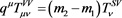, we get

(15)

Here we can identify a low-energy limit given by

Then it is expected that the term in the VV function satisfies

A very interesting aspect, however, is relative to the second contraction

which implies that. In this way the two-point functions SS, VS and VV as well as the one-point ones S and V are involved in these low-energy predictions.

B. Axial indexes

Now let us consider the AP function. The general form is similar to that of SV function

such that

where is a scalar function. It is expected then that, since may not have a pole at. However, the axial current must be proportional to the pseudoscalar one such that we have to get

which implies that, as a consequence of the Ward identity relating the axial and the pseudoscalar fermionic currents.

Now we consider the AA function. Similarly to VV amplitude we have

The Ward identities allow us the identification

As a consequence we have

Again we can identify a low-energy implication

Now we can see that the two contractions lead to

which implies that we have to get. Such that the amplitudes PP, AP, AA, S and V are involved in these low-energy predictions.

C. Axial and vector indexes

Now let us consider the functions having an odd number of. For PV, AS and AV amplitudes we can write

(16)

The tensor carries one vector and one axial index corresponding to vector and axial currents such that we must have the properties dictated by the Ward identities. Contracting the expression (16) with the vector external momenta, and using the Ward identity, we arrive at the result

and it is expected that

A low-energy implication follows

Contracting now the amplitude with the axial vertex momentum, we obtain

and, as a consequence,

or yet

Now since

we have

This expression means that at the left hand side must vanish, which implies that at this kinematical point we have to get also

or in another way

This is the implication analogous to the equal mass case, which is. So, if both Ward identities for the AV function are satisfied then it is predicted that the above combination of PV and AS amplitudes must vanishes at. This prediction is general and not restricted to perturbative solutions. The above results relating PV, AS, PS, and AV amplitudes are consequence of the general structure for these amplitudes in addition to the validity of Ward identities.

At this point, the relevant question is: can we evaluate all the involved perturbative amplitudes so that the expected properties, relations among Green functions, Ward identities and low-energy limits can be satisfied simultaneously? This is our challenge since there are mathematical troubles in the amplitude definitions which must be consistently handled in order to find adequate solutions for the perturbative amplitudes.

5. The Strategy to Handle the Divergences of the Perturbative Calculation

In the preceding sections we have introduced a general interaction Lagrangian and constructed the one-loop amplitudes through the ingredients given by the Feynman rules, for one value of the loop momentum, which may become divergent after integration over all such values. The integration was not taken precisely by the fact that some amplitudes, in that case, will become mathematically undefined quantities and the posterior operations are dangerous since all the physical content of the amplitudes (external momentum dependence) will be present in divergent integrals and then the calculations only become possible if some modifications of the amplitudes are made. Schematically, we have to adopt the following procedure

(17)

where the’s are parameters of the distribution, and the limit which allows to remove the distribution in the finite integrands, connecting the modified expression to the original ones (coming from the Feynman rules), , must be well-known. By assuming the presence of this very general regularization we can manipulate the integrand through algebraic identities since the integrals are now finite.

In order to avoid the problems related with the usual regularization schemes we will adopt an alternative procedure to perform all the necessary calculations in the perturbative amplitudes, including renormalization processes, without modifying the amplitudes as they emerge from the Feynman rules. The procedure is in addition universal in the sense that any amplitude of any theory in any space-time dimension is treated in the same way. Such strategy, proposed and developed by O. A. Battistel originally in Ref. [17] , is founded in a simple idea: to avoid the critical step involved in the regularization process which is the explicit evaluation of divergent integrals.

The implementation of the procedure is simple. The central idea is to write the propagators in a way that the momentum structure is emphasized. The divergences occur because the conditions imposed in the differential equation for the Green functions of the free part are not enough to render the perturbative solutions of the interacting theory convergent. More restrictive convergence conditions would be necessary. So it is possible to separate the part of the propagators which are responsible for the divergences if a decreasing power series is generated. Schematically, we can represent the summation as

where the corresponding integrals have a power counting which decreases as n increases, such that the last term can be convergent. If this is possible then the connection limit can be taken in such term which means to remove the distribution from the integral just because the integration and the limit commute in this case, such that the right hand side can be written as

In this step, it is assumed only the validity of the linearity in the integration process. The last integral can be performed without specifying the regulating distribution and the result must be universal (regularization independent).

According to the space-time dimension more inverse power will be associated to divergences but there always will be a certain power which will correspond to convergent terms. This scenario will be perfect if no physical parameter are present in the potentially divergent terms such that the part which contains the energy-momentum dependence will reside totally in the convergent term. The remaining potentially divergent terms will be, in principle, dependent on the specific regularization. However, there will be properties of them which may be universal too, as we will see in a moment.

In order to implement such procedure we can adopt an adequate representation for a propagator carrying momentum such as

(18)

Note that, as N increases, the convergence becomes better. This identity is very convenient for our purposes. Here is a momentum of an internal line in the loop, and is the mass carried by the corresponding field. In the above identity we have introduced an arbitrary parameter λ with dimension of mass. As it will be shown in the next sections, this parameter gives a precise connection between the divergent and finite parts. It plays the role of a common scale for the divergent and finite parts of the corresponding Feynman integrals. The value taken for N in a Feynman integral, according to the brief discussion above, must be taken as major or equal to the highest superficial degree of divergence of the considered theory or model, if we want to take an unique representation for all involved propagators. Once this representation is assumed, the integration in the loop momentum can be introduced (the last Feynman rule). All the Feynman integrals containing the internal momenta will be present in finite integrals. On the other hand, the divergent ones, which contain only the arbitrary mass scale λ, assume then standard mathematical forms as

The tensorial structure states general properties for such objects. Among such properties, there must be a relation among them such that all the objects above can be reduced to first one. These relations must be independent of the particular regularization.

The set of potentially divergent terms can be then separated in two classes of objects; the irreducible ones and those which are convenient combinations of terms having the same degree of divergences but different tensorial structures. Such objects are not really integrated as we will show in a moment, so that no divergent integrals need in fact to be solved. In renormalizable theories the irreducible objects can be absorbed in the reparametrization of the theory and in nonrenormalizable models they will be directly adjusted to phenomenological parameters in the parametrization of the model, in each specific level of approximation considered. More details about these aspect of the procedure will be presented in a moment when the chosen amplitude is evaluated.

In order to make clear the point stated above, as an example, for the present case the fermion propagator can be written as

(19)

This expression is obtained by taking in Equation (18) and performing the summation over index j. This value for N is relative to the highest (superficial) degree of divergence which we have to consider. In present case such value corresponds to the one-point vector or axial Green function. Note that the expression above is independent of the arbitrary scale parameter λ. This can be easily checked by verifying that. The presence of the arbitrary scale parameter is required to preserve the arbitrariness involved in the separation of terms having different power counting in the loop momentum. It is easy to verify, within the context of traditional strategies, that in this type of separation there is an arbitrariness.

By using the above form for the fermionic propagator we will have the desirable property for all one-loop amplitudes in which all the dependence on the internal momenta will be in present in finite integrals. However, unnecessary algebraic efforts can be avoided noting that in cases of lower than N divergence degree we can (before or after taken the integration) turn back one or more steps in the above expansion of the propagator until the dependence on the internal momenta is located in finite integrals. This point will become clear in what follows. Let us now evaluate the one-loop amplitudes involved in our investigation within the context of the above described procedure and then show many other aspects of the referred strategy.

6. Explicit Calculations of One and Two-Point Functions

We start, following the strategy described in the preceding section, by considering the evaluation of the simplest ones but those having the higher divergence degree in the theory which is the one-point scalar, vector and axial fermionic Green functions defined in (4). Let us consider one of them in details, in order to illustrate the procedure. We first write

(20)

where. Since the divergence degree acquired will be linear for the first term in (20), we choose in the expression (18) so that

or, since the odd terms will be ruled out after the integration, we write

(21)

For the second term the same expression for the propagator can be used. However, in order to avoid unnecessary algebraic efforts we can note that it is equivalent to adopt the expression (18) corresponding to. This is a general statement. If a higher (than the superficial degree of divergence) value for N is assumed the result can always be reduced to the one corresponding to the lowest possible one. Then we get

(22)

Adding the two terms, (21) and (22), in order to obtain the vector Green function,

so that the dependence on the arbitrary internal momentum is located in finite integrals. The divergent terms will not contain physical quantities since λ is an arbitrary parameter which will play the role of a common scale for the divergent and finite parts. We can then introduce the integration on both sides in order to obtain the physical amplitude. It is certainly correct to say that

The integration of the (finite) integrals obtained reveals an exact cancellation. This means that we can state the formal relation

(23)

where we have defined

(24)

With the same ingredients we get

(25)

Note the completely arbitrary character of the results. Analogously, for the S function we can state that

(26)

The integration of the (finite) integral obtained reveals that the formal relation can be stated

(27)

with

The function is identically zero due to the Dirac traces properties.

Following the same procedure, in the same spirit adopted above, we get the following results for the two-point functions

(28)

(29)

(30)

(31)

(32)

(33)

(34)

(35)

(36)

where we introduced the functions

In the above expressions (and in future ones), the arguments of such functions are omitted by simplicity.

At this point it is interesting to note that the mathematical forms of the amplitudes presented above preserve all the arbitrariness involved in this type of calculations. In addition, no modification, relative to the implication of Feynman rules, has been introduced, as is usual in regularization prescriptions. On the other hand, since only finite integrals have been solved, the results corresponding to particular regularizations can be obtained directly from the above expressions. For this purposes it is only necessary to perform the integration of the two divergent objects present in the expressions; and. These two objects remain unspecified at this point and the remaining freedom resides precisely on the values assumed by them, if we look at the amplitudes as regularized quantities, as usual. For the operations made until now, it was assumed only the validity of the linearity in the integration operation in Feynman integrals, in spite of the divergent character. Let us now analyze the obtained results.

7. Verification of Relation among Green Functions

Before any analyses we have to verify the consistency of the performed operation. We must test the obtained results concerning the maintenance of the linearity in the integration operation. In our problem, a crucial test is the verification of the relations among Green function stated in the section III. We start by the VV function, Equation (34). Contracting with external momentum

The second term can be identified as, by comparing with the expression (30). On the other hand it is simple to see that

so that we have obtained,

which is in accordance with the expectation stated by the expression (5).

For the SV function, Equation (30), we first state

Using the relation between finite functions

which reduces the function to, as well as

we write

which is the desired result stated through the expression (6), given the expressions (27) and (28) to S and SS amplitudes.

Contracting the expression for the AA amplitude, Equation (35) we get

which implies that

by comparing with the expression (23) and (33) to the functions V and PA.

By contracting the obtained expression, Equation (33), we get

Again we reduce the function to the function and the result is the expected property

The contraction, Equation (31), is obtained, which is the correct result since the functions P and PS involved in the corresponding identity are both zero.

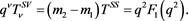
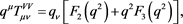
By contracting the expression (36) with the external momentum we get

Comparing with the expression (31) and (25) for the AS and A functions, we conclude that

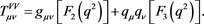
which means that the relation is preserved. Now we contract with the axial index,

(37)

Using the relation among the finite functions

we obtain

Now looking at the expression above, in order to identify the involved one-point A functions, Equation (25), it is first necessary to use a 2D version of the Schouten identity

It is easy then to identify the one and two-point amplitudes such that

Differently from the preceding cases, here the expected relation is only obtained if the condition is satisfied. This is a very important aspect, because if the attributed value for this quantity is different from the above one, the linearity of the integration operation is broken. Obviously, this is related to the anomalous term in the AV anomaly. Let us consider this object in a more detailed way. First we write

This is a difference between two logarithmically divergent structures. However, using, one more time, the linearity of the integration operation, we can add and subtract in the numerator of the first term to obtain a cancellation of the divergent part. The result is finite and completely well defined

Note that this quantity represents the trace of the object. We concluded the verification of the relevant relations among Green functions. The manipulations and calculations made until now are consistent to the linearity in the integration operation given the fact that the above obtained condition is fulfilled in a way independent of the particular prescription.

8. Ward Identities and Divergent Object

In the preceding section we verified if the relations established to perturbative 1-loop amplitudes have been preserved by the performed operations in the context of adopted strategy. All relations among Green functions are preserved without any condition for the value of the divergent quantities present at the expressions for the amplitudes within the context of the adopted mathematical language, except the one corresponding to the contraction of the AV amplitude with the external momentum with the axial index. This means that all regularizations are capable to fulfill such relations independent of the value attributed to the divergent objects, except that for the axial index of the AV amplitude where a specific (but reasonable) property is required. This exception character is obviously related to the axial anomaly, as we will discuss in what follows.

At this point we must consider the crucial question in perturbative calculations: are the results consistent with the symmetry content of the model? In this case this means to satisfy the Ward identities. The problem is simple in the sense that we have at our disposal only two unspecified quantities; and. Therefore, we must question ourselves about the possible values for these quantities in order to get the symmetry relations satisfied, if such values really exist. Our job is easy due to the previous section.

Let us start by the amplitudes having two Lorentz indexes. The relation (5)

reveals in a very transparent way that the Ward identity corresponding to the divergent of the vector current will be satisfied only if the two first term on the right hand side are absent. Following the usual interpretation, the amplitudes require a regularization. So the question is: Is there a regularization which is capable to do the one-point V function identically zero? Looking at the expression

we see that apparently two options are possible. The first is to choose the arbitrary internal momentum as zero. Following this procedure we are accepting that the perturbative amplitudes are ambiguous quantities and the ambiguities need to be fixed by convenient choices case by case. Furthermore, we cannot take the values for and simultaneously zero in the Equation (5). The second option is to select a regularization which gives

(38)

This is possible within the context of dimensional regularization, for example. So, without questioning if this is consistent, for a while, we accept this condition as a Consistency Relation (CR), just because it seems that we do not have another option at this point. As a consequence the required Ward identities

are preserved. The same analysis for the AA amplitude leads us to the same conclusion. In this case the reason is obviously related to the fact that with the CR assumption.

Now we take the AV function, given by (after assuming the CR),

and then, showing that the Ward identity for the vector index is preserved.

Now we consider the axial vector index. It is immediate to see that

showing that the axial-vector Ward identity is violated due to the presence of the nonambiguous finite term, which is the well-known anomalous term. This is not a surprising fact just because we have yet established that if we will have a term which breaks the linearity of the integration operation, given rise to an anomalous term. Therefore, it is simple to see that there is no solution for this dilemma. The required results and are not possible simply because a tensor cannot be identically zero and, at the same time, having a nonzero trace. The anomalous term is a consequence of the values which is also not consistent just because it leads to the violation in the linearity of the integration operation as well as because there is no fair procedure which can make the. Note that in the Schouten identity

there are only two possibilities: both objects and are zero or both nonzero. One can say that, in order to state that, we have, in fact, calculated a divergent integral. However, note that we can consider the expression for the AV amplitude in a one step before the Equation (36), where the integration has not yet been taken. Then we can use the identity

where means without the integration sign. The last term on the right hand side is

It is easy to accept that this is equal to

Then, we introduce the last Feynman rule. The integration of the two imediately above quantities must be identified as being equivalents, due to the linear character of the integration operation. So, it seems that the zero value attributed to the object cannot be correct since is clearly nonzero. The more surprising fact is that even if we close our eyes for these facts, this is not enough to render the perturbative amplitudes consistent quantities. In order to see this it is necessary only to analyze the Ward identities for the amplitudes having one Lorentz indexes.

Looking at the relations among Green functions

it is simple to see that there is only one condition which is capable to guarantee the preservation of Ward identities which is the identically zero value for the S one-point functions. This means that it is required that. This is an impossible requirement. There is no regularization or fair calculation capable to fulfill this requirement. The implication is

for any fair procedures. This is not the complete history. Let us next analyze the low-energy limits.

9. Low-Energy Limits

In the section IV we obtained low-energy predictions for the amplitudes stated as a consequence of Ward identities and the general tensorial aspects of the amplitudes. In the previous section we concluded that it is not possible to fulfill the conditions required in order to obtain all amplitudes satisfying their Ward identities. In this section we will complete our investigation by making an additional exercise. Let us accept that the required conditions are satisfied in a hypothetical way, and verify the predicted low-energy limits. This exercise is necessary just because, otherwise, the verification of low-energy limit is immaterial, since such results have been obtained by assuming the validity of the symmetry relations. Let us, in a first moment, assume that a regularization, which is capable to obtain

does exist (without believing that this is really possible). The gives us and gives us. And then we can ask ourselves: Are the predicted low-energy limits preserved? It is expected, through these assuptions, that a violation ocurr in the AV amplitude. Just due to this it is called anomalous. But will violations ocurr only for the AV amplitude?

We start by considering the SV amplitude. The obtained result is

revealing that the expect property is, obviously, preserved. On the other hand, the associated SS function, after the assumptions made above, is given by:

obtained by simply removing the quantities in the obtained expression, will be not consistent with the predicted low-energy limit due to the fact that

and, therefore, , which means that even if the S terms are removed “by hand” in order to fulfill the Ward identity relating the SV and SS functions the low-energy limit is not satisfied.

The same occurs with the AP and PP relation. While the low-energy limit for AP function is naturally preserved, the prediction for the PP function will be not fulfilled, since even if the Ward identity violating terms are removed “by hand” we will get.

Finally, let us consider the amplitudes which are odd tensors. The low-energy limit

is predicted to be zero. Therefore, it is not preserved as well as in the case of SV and AP.

The violation involved in the above considered limit is expected, just because it is precisely the one related to the AV axial anomaly problem. However, it is important to note that, at the same scenario, we have other violations in the predicted low energy limits, which are usually not expected. Due to this reason, the immediately above considered case do not have a status of exception. If all the amplitudes are treated in the same way, the violation in the predicted low energy behaviour, is the rule and not an exception. The conclusion is transparent: the interpretation given for the perturbative amplitudes as quantities to be regularized cannot give us consistent results in a wide sense.

10. Final Remarks and Conclusions

Quantum Field theory has obtained very important successes in the accordance between theoretical predictions and experimental data. Such successes have been obtained through perturbative solutions where the amplitudes are taken as quantities to be regularized and after renormalized. Due to this reason only renormalizable quantum field theory are part of the referred successes. It is a fact. However, there are very intriguing aspects in the adopted procedures, relative to the interpretation of the perturbative amplitudes as regularized quantities. In the present work we developed a detailed investigation in order to show some of such aspects. The dimension adopted for the space-time is just to give us the simplest scenario from the mathematical point of view, but the points discussed here are present in all space-time dimensions in all theories and models. The authors of the present work have been made a considerable effort in order to understand in the deepest way the questions relative to the consistency in perturbative calculations. Part of such efforts resulted in a simple and transparent procedure to make the required manipulations and calculations where it is possible to avoid the use of regularizations in intermediary steps as well as a complete systematization of the procedures has been obtained. After this it is simple to identify some situations where it is apparently not possible to obtain the required consistency. The simple investigation presented here exhibits some of such situations. The required calculations are very simple. In spite of this, the conclusions are powerful.

The main point of our work is the requirement of the validity of the linearity in integration operation in Feynman integrals, in spite of the divergent character involved, at any stage of the calculations. It seems so simple and obvious to require the preservation of this absolutely fundamental mathematical property in the operations made in perturbative calculations of quantum field theory, but this is a difficulty for all regularization procedures, specially for the dimensional regularization. It is not usual to emphasize this aspect just because it is not usual to verify if the obtained results are consistent with such requirement. Given the presence of mathematical indefinitions at the loop amplitudes, the preservation of the linearity in the manipulations made in Feynman integrals is not automatic. Because of this, such property can be used as a powerful constrain in the searching for the consistent interpretation of the perturbative amplitudes. It is certainly a very difficult situation to state physical consequences of a theory through the solutions which breaks the linearity in the integration operation. A simple but important consequence is that it is possible to show that all anomalous terms are linearity breaking, as we have shown in the considered case. In a consistent calculation, such terms cannot be present. It is possible to identify, in a very clear way, the step where the anomalous term emerge, just because it is precisely where the referred linearity is broken. In the expression for the AV amplitude, Equation (37), we have the term. Then we used an identity, which can be stated at the level of the integrands,

and then two terms appeared. The first term, in the right hand side, will generate two one-point axial amplitudes while the second one will add to the term, coming from the finite part. If one adopts a prescription where is zero, like dimensional regularization does, then the remaining two terms will not arise so that the factor will not be cancelled breaking the axial Ward identity. However, the above identity is correct and the term cannot be made zero at any fair procedure. Its value cancels in an exact way the factor, recovering the linearity or the relation among Green functions. In fact, the generation of the anomalous term in all anomalous (divergent) amplitudes occurs in a completely similar way (work along this line is presently in preparation). Note that the above identity can be stated for the integrands of the three terms. Therefore, before the implementation of the last Feynman rule, which is the integration in the loop momentum. Because of this, the violation of the linearity, materialized at the relations among Green functions in our approach, occur precisely at this step if the identity is violated after the integration, usually made by using a regularization.

The correct procedure, given such analyses, is to obtain a nonzero value for the object since the identity above does not admit another result. In fact, in order to attribute a zero value for the object it is necessary to violate first the general property

for, in a second step, violate also the linearity. Explicitly, we have

The same result can be obtained in the presence of any regulating function. The result within the context of dimensional regularization can be understood if we rewrite the above object in a different way

It is a surface term and so is taken as zero in dimensional regularization, by construction. But this assumption is clearly not compatible with symmetric integration and linearity, as shown above. In addition, this make possible that the trace can be obtained as nonzero for an identically zero tensor. On the other hand, it is very simple to verify that

for any which makes the integrand convergent. The result is clearly convenient. It works like a Consistency Relation in perturbative calculations just because saves, among others, the gauge invariance of the polarization tensor in the quantum electrodynamics in two dimensions but, given the above arguments, it is clearly unfair. Despite of this it is not enough to save other symmetry relations like

just because, the preservation of these symmetry relations requires that

This would be a completely absurd idea. In dimensional regularization we have a nonzero value and a pole in the value. In the most common regularizations, like Pauli-Vilars [18] , we have a. Therefore, the result, in spite of the fact that is very convenient, obtained in dimensional regularization by construction, cannot save all situations at all. This execise made in other space-time dimensions will require that all divergent quantities must be identically zero.

The low-energy limits analysis reveals an additional aspect. Even if the Ward identities are preserved by assuming the contradictory results, , and, the low-energy limits predictions for the SS and PP functions are not correct. In this sense, even if we accept that the AV Axial Ward identity must be violated, in order to save the low-energy limit, this situation will be not an exception but part of a rule.

The conclusion is clear: it is not possible to give a consistent interpretation for the perturbative amplitudes as regularized quantities. In other words, do not exists a (honest or not) regularization procedure which is capable to leads to the expected (consistent) results.

All the conclusions stated here are constructed as a consequence of the application of a very careful procedure, which is, in addition, very simple in such a way that all the results presented here can be easily checked. The implications, however, seem to be very important since many phenomenological implications are linked to these fine tuning aspects of the perturbative calculations in quantum field theory. Many controversies aroused in recent years are deeply related to the questions discussed here.

Finally, at this point, it is unavoidable to formulate the question: Can we believe that it is possible to construct an adequate interpretation for the perturbative amplitudes without considering them as quantities to be regularized? The answer seems to be: yes. A work following this line of reasoning is presently in preparation.

Acknowledgements

L. Ebani acknowledge a grant from CNPq/Brazil.

Conflicts of Interest

The authors declare no conflicts of interest.

References

[1]	Adler, S. (1969) Physical Review, 177, 2426-2438. https://doi.org/10.1103/PhysRev.177.2426
[2]	Bardeen, W.A. (1969) Physical Review, 184, 1848-1857. https://doi.org/10.1103/PhysRev.184.1848
[3]	Bell, J.S. and Jackiw, R. (1969) Nuovo Cimento A, 60, 47-61. https://doi.org/10.1007/BF02823296
[4]	Jackiw, R. (2000) International Journal of Modern Physics B, 14, 2011-2022. https://doi.org/10.1142/S021797920000114X
[5]	Treiman, S.B., Jackiw, R., Zumino, B. and Witten, E. (1985) Current Algebra and Anomalies. World Scientific, Singapore. https://doi.org/10.1142/0131
[6]	Gross, D. and Jackiw, R. (1972) Physical Review D, 6, 477-493. https://doi.org/10.1103/PhysRevD.6.477
[7]	Gerstein, L.S. and Jackiw, R. (1969) Physical Review, 181, 1955-1963. https://doi.org/10.1103/PhysRev.181.1955
[8]	Bertlman, R.A. (1996) Anomalies in Quantum Field Theory. Clarendon Press, Oxford.
[9]	’t Hooft, G. and Veltman, M. (1972) Nuclear Physics B, 44, 189-213. https://doi.org/10.1016/0550-3213(72)90279-9
[10]	Bollini, C.G. and Giambiagi, J.J. (1972) Physics Letters B, 40, 566-568. https://doi.org/10.1016/0370-2693(72)90483-2
[11]	Ashmore, J.F. (1972) Nuovo Cimento Letters, 4, 289-290. https://doi.org/10.1007/BF02824407
[12]	Sutherland, D.G. (1966) Physics Letters, 23, 384-385. https://doi.org/10.1016/0031-9163(66)90477-X
[13]	Sutherland, D.G. (1967) Nuclear Physics B, 2, 433-440. https://doi.org/10.1016/0550-3213(67)90180-0
[14]	Veltman, M. (1967) Procedure Royal Society A, 301, 107. https://doi.org/10.1098/rspa.1967.0193
[15]	Battistel, O.A., Fonseca, M.V.S. and Dallabona, G. (2012) Physical Review D, 85, 085007. https://doi.org/10.1103/PhysRevD.85.085007
[16]	Gnendiger, C., et al. (2017) European Physical Journal C, 77, 471. https://doi.org/10.1140/epjc/s10052-017-5023-2
[17]	Battistel, O.A. (1999) A New Strategy to Manipulate and Calculate Divergencies in TQC. PhD Thesis, Universidade Federal de Minas Gerais, Brazil.
[18]	Pauli, W. and Villars, F. (1949) Review Modern Physics, 21, 433. https://doi.org/10.1103/RevModPhys.21.434