Received 13 May 2016; accepted 24 July 2016; published 27 July 2016

1. Introduction
Over the last decades, there has been a great deal of interest and significant progress in the study of nonlinear plasma theories and many of works and researches in plasma physics devote much attention to these theories. The nonlinear theories include a large number of effects and phenomena such as the nonlinear coherent structures as shock waves, solitary waves (solitons), vortices, etc.
The collective electrical and magnetic properties of plasmas could produce interactions that take the place of collisions and permit shocks and solitons to form. A shock wave is a sudden transition (a type of propagating disturbance) in the properties of a fluid medium (liquid or gas), involving a difference in flow velocity across a narrow (ideally, abrupt) transition. In high-energy density physics, nearly any experiment involves at least one shock wave. Such shock waves may be also produced by applying pressure to a surface or by creating a collision between two materials.
Nonlinear effects in plasmas occur when a large amplitude wave is excited by an external means. Soliton (shock) waves are formed as a result of a balance between the nonlinearity and dispersion (dissipation) of the medium. For example, the dispersion in the ion acoustic wave can be counter-balanced by nonlinearity and an ion acoustic soliton can propagate. From the mathematical point of view, solitons are the stationary solutions to the Korteweg-de Vries equation:
 (1)
(1)
where  is a function of position x and time t. Some historical events and discoveries led to the soliton theory and Equation (1) is not the only equation that has solitonic solution. The sine-Gordon and the nonlinear Schrödinger equations are among them. The solutions to the Equation (1) are traveling wave with constant profile in time and they describe the different types of models in various branches of physics and natural science (for instance, Equation (1) is modeled to describe the waves on shallow water surfaces).
As mentioned, Equation (1) may arise in the study of such diverse physical systems as fluids and plasmas. In plasma ambient, Equation (1) may be due to the balancing between nonlinearity and dispersion and for this reason its study is of special interest.
One of the possible approaches to study of the nonlinear effects is the so-called reductive perturbation technique [1] - [5] . This technique is widely employed to investigate the asymptotic behavior of nonlinear excitations and is more convenient to study of small-amplitude nonlinear perturbations, or to treat of plasma waves in a state very close to thermodynamic equilibrium.
Another successful approach to study of the electrostatic solitons and shock waves has been the Sagdeev Potential (SP) or Pseudo Potential (PP) method. The SP is one particular notion that has become immensely important in soliton and shock research [6] . The main advantage of this method over reductive perturbation technique is that, it is appropriate for arbitrary amplitude waves and one can derive all the soliton results of perturbation methods and compare it with the exact results obtained by the SP method [7] .
In the present work, our aim is to compute the soliton width (SW) for an ion acoustic solitary wave propagated in a cold plasma. The computation is based on analogy between pseudo-particle in PP well and real particle in conservative potential well. Knowing the angular frequency of (small) oscillation of real particle about its equilibrium position and comparing this with corresponding quantity in the plasma system, one attains a formula to compute the SW. To understand briefly, the SW is defined as spatial length corresponding to a (complete) spatial oscillation of psuedo-particle in the PP well; comparing this with the definition of period of temporal oscillation for real particle in the well, the computation is straightforward. Also, for better understanding of the changes, the graph of the width function is visualized, with the help of numerical plotting (computer algebra).
The work is organized as follows:
The model and the main calculation are presented in the next section, and conclusions are given in the last section.
2. The Soliton Width as a Function of the Mach Number
We will consider a one dimensional model for propagation of ion acoustic wave in a cold plasma. The solitary wave is generated by spatial oscillation of electrostatic potential  which is the so-called psuedo-particle. The wave is travelling to the left in the (to say) x direction with a constant speed
 . Therefore, in the wave- frame position, the SP is given by [8] :
 (2)
(2)
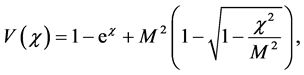
This PP is subjected to the boundary condition , and the following dimensionless parameters are used

where  to be electron temperature,
  is the ion Debye length and M is the Mach number.
The form of the PP would determine whether soliton like solutions may exist or not. The conditions for the existence of solitary waves are:
where  is the maximum value of
  beyond which the PP becomes imaginary1 and it is often called amplitude of the soliton (or shock). By virtue of above conditions, it is easily to show that the values of the Mach number are confined to the interval
 (3)
(3)
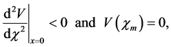
It may be useful to plot the graph of the PP (2) versus its argument . The graph is illustrated in Figure 1 for three values of M. As the figure shows, the depth of the potential well and amplitude of the soliton increase with increasing Mach number.
The PP (2) satisfies the energy condition:
 (4)
(4)
which is analogous to the principle of energy conservation
![]()
for a real particle of mass m moving in a (conservative) potential![]() . In view of this analogy, Equation (4) can be regarded as an energy integral of moving pseudo-particle of unite mass, pseudo-position
. In view of this analogy, Equation (4) can be regarded as an energy integral of moving pseudo-particle of unite mass, pseudo-position![]() , pseudo- velocity
, pseudo- velocity ![]() and pseudo-potential
and pseudo-potential![]() . Hence, by the following replacements:
. Hence, by the following replacements:
![]()
one can obtain similar formulas and results in the plasma system, as discussed below.
We know that for a real particle moving in the potential![]() , the angular frequency of small oscillations
, the angular frequency of small oscillations![]() , about the equilibrium position (a minimum at
, about the equilibrium position (a minimum at![]() ) is given by
) is given by
![]() (5)
(5)
![]()
Figure 1. Psuedo-potential curves V(χ) corresponding to three values of M2 = 1.2, 1.3, 1.4.
and as a result, the period of oscillation motion T becomes
![]() (6)
(6)
The natural question, then, is what conclusions can be drawn from this for our plasma system, more clearly, what quantities are given by similar formulas which are obtained by the above replacements in (5) and (6), that is
![]() (7)
(7)
and
![]() (8)
(8)
where we also use ![]() and the two replacement
and the two replacement ![]() in (5),
in (5), ![]() in (6)2.
in (6)2.
It is easily to check that ![]() has the dimensions of the Length, and in below, we see that
has the dimensions of the Length, and in below, we see that ![]() is SW.
is SW.
We first remind the following definitions:
T: a time interval corresponding to one complete temporal oscillation of real particle (in the well).
On the other hand the width of the solitary wave is equal to the length that disturbance of the solitary wave takes place, or in SP terminology,
SW: a distance interval corresponding to one complete spatial oscillation of pseudo-particle (in the PP well), thus, it is natural to drawing the result
![]() (9)
(9)
To use the above formula, we need to know the point![]() , that is minimum of PP. This is given by vanishing of the first derivative of PP (2), namely
, that is minimum of PP. This is given by vanishing of the first derivative of PP (2), namely
![]() (10)
(10)
solving this equation for![]() , we get
, we get
![]() (11)
(11)
where W is the Lambert function. Substituting ![]() into the second derivative
into the second derivative
![]() (12)
(12)
and using Equation (9), we obtain the final expression for the SW as function of the Mach Number, that is
![]() (13)
(13)
Due to the presence of Lambert function, we have no clear idea of the behavior of the width function (13), then it is instructive to graph the function. Because of the transcendental form of the function, we have to use the numerical plotting and the corresponding graph is illustrated in Figure 2. It represents a monotonically decreasing function of M. The function takes on arbitrarily large values when![]() , and decreases rapidly over the (allowable) range
, and decreases rapidly over the (allowable) range![]() .
.
As mentioned, the soliton width is the length of a complete sweep of the pseudo-particle in the potential well and as is clear from the Figure 1, the potential well corresponding to the larger values of M is more narrow than
![]()
Figure 2. The graph of the soliton width λs versus M: rapidly monotonic decreasing function.
the smaller one, then, the solitons corresponding to larger M have shorter width.
In order to have a quantitative measure of the changes of the width function, let us compute the ratio
![]()
where and ![]() are near the upper and lower bounds of M respectively, that is
are near the upper and lower bounds of M respectively, that is![]() ,
,![]() . From Figure 2, one finds
. From Figure 2, one finds
![]()
inserting these values in to the ratio, we obtain
![]()
This number is the average decreasing rate of the width per mach number, that is the change in the width divided by the change in Mach number. The negative sign indicates the decreasing nature of the function. As it is evident the amount of decreasing is relatively large.
In the above discussion, the width changes were described in terms of the Mach number itself, but, due to definition of the Mach number![]() , the following easy corollary can be deduced:
, the following easy corollary can be deduced:
1) A positive (negative) change in the soliton wave velocity ![]() leads to a negative (positive) change in the SW, and
leads to a negative (positive) change in the SW, and
2) A positive (negative) change in the ratio (![]() ) leads to a positive (negative) change in the SW.
) leads to a positive (negative) change in the SW.
In the end of this section, it is necessary to say that our ability to plot the width function ![]() (as continues function) is because of the analytic form of the SP (2). Indeed, the method presented here may be employed for any SP of analytic form [9] . When the SP has not analytic form, there is no such ability, but we may still calculate numerically
(as continues function) is because of the analytic form of the SP (2). Indeed, the method presented here may be employed for any SP of analytic form [9] . When the SP has not analytic form, there is no such ability, but we may still calculate numerically ![]() at each allowable equilibrium (a minimum) position. This is based on estimation of equilibrium position and substituting into the second derivative of SP. In this case, one has a (discrete) point diagram, instead of a continues curve. One such computation has been represented in [10] for an electron-positron plasma including stationary ions in the background.
at each allowable equilibrium (a minimum) position. This is based on estimation of equilibrium position and substituting into the second derivative of SP. In this case, one has a (discrete) point diagram, instead of a continues curve. One such computation has been represented in [10] for an electron-positron plasma including stationary ions in the background.
3. Conclusions and Results
The shock and soliton waves occur most likely because of the nonlinear disturbances, namely discontinuities in various variables as energy density, pressure, temperature, etc, in plasmas and other mediums. In addition to amplitude and velocity of disturbance, the determination of spatial scales within the collision less shock or soliton may be of particular interest. For example, for a shock disturbance ![]() which obeys the Burgers equation
which obeys the Burgers equation
![]() (14)
(14)
with the initial condition
![]() (15)
(15)
it can be shown [11] that the width and speed of the shock are respectively
![]()
In the case of ion acoustic wave which is mediated by electric potential in the plasma, the width of the shock or soliton may be particularly important in its relation to the width of the electrostatic potential drop across the shock.
In this work, the PP approach is employed to calculate the width of (one dimensional) ion acoustic solitary wave propagating in a cold plasma. The calculation shows that the soliton width is a continuous function of the Mach number and the function is expressed in terms of the Lambert function. Because of transcendental form of the width function, we have to use the numerical method (computer algebra) to graph of the function over the (short) allowable range of the Mach number (![]() ). The graphical representations help us to understand the behavior of the width function. The main feature of the graph is monotonic rapidly decreasing one, such that the average rate of change is about 82 unit of the length per Mach number. Contrary to the width, the amplitude of solitary wave is an increasing function of the Mach number.
). The graphical representations help us to understand the behavior of the width function. The main feature of the graph is monotonic rapidly decreasing one, such that the average rate of change is about 82 unit of the length per Mach number. Contrary to the width, the amplitude of solitary wave is an increasing function of the Mach number.