On the Construction of Analytic-Numerical Approximations for a Class of Coupled Differential Models in Engineering ()
1. Introduction
Coupled partial differential systems with coupled boundary-value conditions are frequent in different areas of science and technology, as in scattering problems in Quantum Mechanics [1] - [3] , in Chemical Physics [4] - [6] , coupled diffusion problems [7] - [9] , modelling of coupled thermoelastoplastic response of clays subjected to nuclear waste heat [10] , etc. The solution of these problems has motivated the study of vector and matrix Sturm- Liouville problems, see [11] - [14] for example.
Recently [15] [16] , an exact series solution for the homogeneous initial-value problem
 (1)
(1)
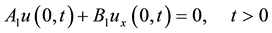 (2)
(2)
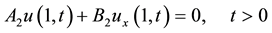 (3)
(3)
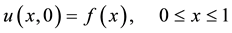 (4)
(4)
where ![]() and
and ![]() are a
are a ![]() -dimensional vectors, was cons-
-dimensional vectors, was cons-
tructed under the following hypotheses and notation:
1. The matrix coefficient ![]() is a matrix which satisfies the following condition
is a matrix which satisfies the following condition
![]() (5)
(5)
where ![]() denotes the set of all the eigenvalues of a matrix
denotes the set of all the eigenvalues of a matrix ![]() in
in![]() . Thus,
. Thus, ![]() is a positive stable matrix (where
is a positive stable matrix (where ![]() denotes the real part of
denotes the real part of![]() ).
).
2. Matrices![]() , are
, are ![]() complex matrices, and we assume that the block matrix
complex matrices, and we assume that the block matrix
![]() (6)
(6)
and also that the matrix pencil
![]() (7)
(7)
Condition (7) is well known in the literature of singular systems of differential equations, see [17] , and involves the existence of some ![]() so that matrix
so that matrix ![]() is invertible. In this case, matrix
is invertible. In this case, matrix ![]() is invertible with the possible exception of at most a finite number of complex numbers
is invertible with the possible exception of at most a finite number of complex numbers![]() . In particular, we may assume that
. In particular, we may assume that![]() .
.
Using condition (7) we can introduce the following matrices ![]() and
and ![]() defined by
defined by
![]() (8)
(8)
which satisfy the condition![]() , where matrix
, where matrix ![]() denotes, as usual, the identity matrix. Under hypothesis (6), is it easy to show that matrix
denotes, as usual, the identity matrix. Under hypothesis (6), is it easy to show that matrix ![]() is regular (see [18] for details) and we can
is regular (see [18] for details) and we can
introduce matrices ![]() and
and ![]() defined by
defined by
![]() (9)
(9)
that satisfy the conditions![]() .
.
Under the above assumptions, the homogeneous problem (1)-(4) was solved in [15] [16] in two different cases:
(a) If we consider the following hypotheses:
![]() (10)
(10)
Then, if the vector valued function ![]() satisfies hypotheses
satisfies hypotheses
![]() (11)
(11)
with the additional condition:
![]() (12)
(12)
where a subspace ![]() of
of ![]() is invariant by the matrix
is invariant by the matrix ![]() if
if![]() , we can construct an exact series solution
, we can construct an exact series solution ![]() of homogeneous problem (1)-(4). This construction was made in Ref. [15] .
of homogeneous problem (1)-(4). This construction was made in Ref. [15] .
(b) If we consider the following hypotheses:
![]() (13)
(13)
Then, if the vector valued function ![]() satisfies the hypotheses
satisfies the hypotheses
![]() (14)
(14)
under the additional condition:
![]() (15)
(15)
then we can construct an exact series solution ![]() of homogeneous problem (1)-(4). This construction was made in Ref. [16] .
of homogeneous problem (1)-(4). This construction was made in Ref. [16] .
Observe that under the different hypotheses (a) and (b), the exact solution of problem (1)-(1) is given by the series
![]() (16)
(16)
where, under hypothesis (a), the value of ![]() is given by
is given by
![]() (17)
(17)
and ![]() is the set of eigenvalues
is the set of eigenvalues![]() , where
, where ![]() is the solution of the equation
is the solution of the equation
![]() (18)
(18)
with an additional solution ![]() if
if
![]() (19)
(19)
and under hypothesis (b), the value of ![]() is given by
is given by
![]() (20)
(20)
and ![]() is the set of eigenvalues
is the set of eigenvalues![]() , where
, where ![]() is the solution of the equation
is the solution of the equation
![]() (21)
(21)
with an additional solution ![]() if
if
![]() (22)
(22)
Under both hypotheses (a) and (b), the value of![]() ,
, ![]() and
and ![]() are given by
are given by
![]() (23)
(23)
![]() (24)
(24)
and
![]() (25)
(25)
taking ![]() in Formulaes (23)-(25) if we consider hypothesis
in Formulaes (23)-(25) if we consider hypothesis![]() .
.
The series solution of problem (1)-(4) given in (16) presents some computational difficulties:
(a) The infiniteness of the series.
(b) Eigenvalues ![]() are not exactly computable because Equation (18) (or Equation (21) under hypothesis
are not exactly computable because Equation (18) (or Equation (21) under hypothesis ![]() holds) is not solvable in a closed form, although well known and efficient algorithms for approximation, see references [13] [19] [20] .
holds) is not solvable in a closed form, although well known and efficient algorithms for approximation, see references [13] [19] [20] .
(c) Other problem is the calculation of the matrix exponential, which may present difficulties, see [21] [22] for example.
For this reason we propose in this paper to solve the following problem:
Given an admissible error ![]() and a bounded subdomain
and a bounded subdomain![]() ,
,![]() . How do we construct an approximation that avoids the above-quoted difficulties and whose error with respect to the exact solution (16) is less than
. How do we construct an approximation that avoids the above-quoted difficulties and whose error with respect to the exact solution (16) is less than ![]() uniformly in
uniformly in![]() ?
?
This paper deals with the construction of analytic-numerical solutions of problem (1)-(4) in a subdomain![]() ,
, ![]() , with a priori error
, with a priori error![]() . The work is organized as follows: in Section 2 we
. The work is organized as follows: in Section 2 we
construct the approximate solution. In Section 3 we will introduce an algorithm and give an illustrative example.
Throughout this paper we will assume the results and nomenclature given in [15] [16] . If ![]() is a matrix in
is a matrix in![]() , its 2-norm denoted by
, its 2-norm denoted by ![]() is defined by ( [23] , p. 56)
is defined by ( [23] , p. 56)
![]()
where for a vector ![]() in
in![]() ,
, ![]() is the usual euclidean norm of
is the usual euclidean norm of![]() , and the 2-norm satisfies
, and the 2-norm satisfies
![]()
Let us introduce the notation
![]() (26)
(26)
and by ( [23] , p. 556) it follows that
![]() (27)
(27)
2. The Proposed Approximation
Let![]() ,
, ![]() , be and we take an admissible error
, be and we take an admissible error![]() . Observe first that given (24), using Parseval’s identity for scalar Sturm-Liouville problems, see [24] and ( [11] , p. 223), one gets that
. Observe first that given (24), using Parseval’s identity for scalar Sturm-Liouville problems, see [24] and ( [11] , p. 223), one gets that
![]()
Thus, we can take a positive constant![]() , defined by
, defined by
![]() (28)
(28)
satisfying
![]() (29)
(29)
Moreover, by (23), we have
![]()
If we define ![]() by
by
![]() (30)
(30)
we have that
![]() (31)
(31)
On the other hand, we know from (27) that
![]()
where, as![]() ,
, ![]() , we have for
, we have for![]() :
:
![]() (32)
(32)
where
![]() (33)
(33)
Observe that for a fixed ![]() the numerical series
the numerical series ![]() is convergent, because using Lemma 1 of Ref. [15] if hypothesis (a) holds, or Lemma 2 of Ref. [16] if hypothesis (b) holds, one gets
is convergent, because using Lemma 1 of Ref. [15] if hypothesis (a) holds, or Lemma 2 of Ref. [16] if hypothesis (b) holds, one gets![]() ,
, ![]() , and by application of D’Alembert’s criterion for series:
, and by application of D’Alembert’s criterion for series:
![]()
then
![]() (34)
(34)
Taking into account that ![]() and
and![]() ,
, ![]() , it follows that
, it follows that
![]() (35)
(35)
and by (34) there is a positive integer ![]() so that
so that
![]() (36)
(36)
Using (29), (31), (32) and (36), if![]() , we have
, we have
![]()
As eigenvalues![]() , then, for
, then, for ![]() it follows that
it follows that
![]() (37)
(37)
Taking into account that![]() , from (37) one gets that
, from (37) one gets that
![]() (38)
(38)
![]()
![]()
![]() (39)
(39)
We take the first positive integer ![]() so that
so that
![]() (40)
(40)
We define the vector valued function ![]() as
as
![]() (41)
(41)
Using (38) one gets that
![]()
thus
![]() (42)
(42)
Remark 1. Note that to determine the positive integer ![]() we need to check condition (36), which requires
we need to check condition (36), which requires
knowledge the exact eigenvalues![]() . From Ref. [15] [16] it is well know that
. From Ref. [15] [16] it is well know that![]() , then
, then
![]()
and by (35), we can replace condition (36) by take the first positive integer ![]() satisfying
satisfying
![]() (43)
(43)
Approximation ![]() defined by (41) involves computation of the exact eigenvalues
defined by (41) involves computation of the exact eigenvalues![]() ,
, ![]() which is not easy in practice. Now we study the admissible tolerance when one considers approximate eigen- values
which is not easy in practice. Now we study the admissible tolerance when one considers approximate eigen- values![]() ,
, ![]() in expression (41), taking
in expression (41), taking
![]() (44)
(44)
where
![]() (45)
(45)
![]() (46)
(46)
with ![]() defined by (25). Note that
defined by (25). Note that
![]() (47)
(47)
It is easy to see that
![]() (48)
(48)
![]() (49)
(49)
and
![]() (50)
(50)
Replacing in (47) and taking norms, one gets
![]() (51)
(51)
We define ![]() for
for ![]() by
by
![]() (52)
(52)
by applying the Cauchy-Schwarz inequality for integrals and (28), one gets:
![]()
We have
![]()
Taking ![]() satisfying
satisfying
![]() (53)
(53)
it follows that
![]() (54)
(54)
Moreover, working component by component:
![]() (55)
(55)
![]()
![]()
![]() (56)
(56)
Applying the Cauchy-Schwarz inequality for integrals again:
![]() (57)
(57)
and
![]() (58)
(58)
![]()
![]() (59)
(59)
By (55) and taking into account (57) and (58):
![]() (60)
(60)
Note that from the definition of![]() , (52), it follows that
, (52), it follows that
![]() (61)
(61)
then, replacing in (60) one gets
![]() (62)
(62)
We take
![]() (63)
(63)
then, if we define
![]() (64)
(64)
from (54) we have that
![]() (65)
(65)
and from (62) and (53):
![]() (66)
(66)
Using the 2-norm properties, from (66) we have
![]() (67)
(67)
By other hand, we can write
![]()
where taking norm, applying (32) and (33) together the mean value theorem, under the hypothesis![]() , one gets
, one gets
![]()
where
![]() (68)
(68)
Replacing in (51) we obtain
![]() (69)
(69)
where
![]() (70)
(70)
Given ![]() and
and![]() , consider approximations
, consider approximations ![]() of
of ![]() for
for ![]() satisfiying
satisfiying
![]() (71)
(71)
then
![]()
and therefore
![]() (72)
(72)
Remark 2. From (61), and taking into account the definition of ![]() and
and ![]() given in (64), it follows that
given in (64), it follows that
![]()
so that, if ![]() is enough small, it can take
is enough small, it can take ![]() in the computation of
in the computation of![]() .
.
Similarly, can be taken in practice
![]() (73)
(73)
instead of the definition (63).
Approximation ![]() need to compute the exact value of the matrix exponential
need to compute the exact value of the matrix exponential![]() . However, the approximate calculation of the exponential matrix
. However, the approximate calculation of the exponential matrix ![]() can be performed by methods such as those based on the Taylor series, [25] [26] , based on Hermite matrix polynomials, [27] , and other existing methods in the literature, see [22] [23] for example. Suppose we take the matrix
can be performed by methods such as those based on the Taylor series, [25] [26] , based on Hermite matrix polynomials, [27] , and other existing methods in the literature, see [22] [23] for example. Suppose we take the matrix ![]() as an approximation of matrix
as an approximation of matrix![]() , so that
, so that
![]() (74)
(74)
We define the approximation ![]() by:
by:
![]() (75)
(75)
and from (65), (64) and (45) one gets that
![]()
We take
![]() (76)
(76)
and suppose we make the approximation accurate enough satisfying condition
![]() (77)
(77)
Thus, if ![]() satisfies (77) it follows that
satisfies (77) it follows that
![]() (78)
(78)
and from (42), (72) and (78):
![]()
Summarizing, the following results has been established:
Theorem 1. We consider problem (1)-(4) satisfying hypotheses (5), (6) and (7). Let![]() ,
,
![]() . Suppose that the hypothesis (a) is verified, this ensures that there is an exact solution
. Suppose that the hypothesis (a) is verified, this ensures that there is an exact solution ![]() of problem (1)-(4), see Ref. [15] . Let
of problem (1)-(4), see Ref. [15] . Let![]() ,
, ![]() ,
, ![]() ,
, ![]() and
and ![]() be the constant defined by (17), (26), (28), (30) and (68) respectively. Let
be the constant defined by (17), (26), (28), (30) and (68) respectively. Let ![]() and
and ![]() be positive integers satisfying conditions (43) and (40). Let
be positive integers satisfying conditions (43) and (40). Let ![]() be the
be the ![]() -first approximate roots of the equation (18), each one in the interval
-first approximate roots of the equation (18), each one in the interval![]() ,
, ![]() , and let
, and let ![]() be the approximation of the additional solution
be the approximation of the additional solution ![]() to be consider if condition (19) holds.
to be consider if condition (19) holds.
Let ![]() be satisfying (53) and let
be satisfying (53) and let![]() ,
, ![]() ,
, ![]() and
and ![]() be the positive constants defined by (63), (64) and (68) respectively. Suppose that the approximations
be the positive constants defined by (63), (64) and (68) respectively. Suppose that the approximations ![]() satisfy (71), where
satisfy (71), where ![]() is the constant defined by (70).
is the constant defined by (70).
Suppose that the approximations ![]() of matrices
of matrices![]() , for
, for ![]() satisfy that the approximation error is less than
satisfy that the approximation error is less than![]() , where
, where ![]() is a positive constant which satisfies (77). Consider the functions
is a positive constant which satisfies (77). Consider the functions![]() ,
, ![]() defined by (45) and vectors
defined by (45) and vectors![]() ,
, ![]() , defined by (46), joint the vector
, defined by (46), joint the vector ![]() defined by (24) if
defined by (24) if![]() . Then, the vector valued function
. Then, the vector valued function ![]() defined by (75) satisfies
defined by (75) satisfies
![]()
Theorem 2. We consider problem (1)-(4) satisfying hypotheses (5), (6) and (7). Let![]() , and we consider the subdomain
, and we consider the subdomain![]() . Suppose that the hypothesis (b) is verified, this ensures that there is an exact solution
. Suppose that the hypothesis (b) is verified, this ensures that there is an exact solution ![]() of problem (1)-(4), see Ref. [16] . Let
of problem (1)-(4), see Ref. [16] . Let![]() ,
, ![]() ,
, ![]() and
and ![]() be the constant
be the constant
defined by (20), (26), (28) and (68) respectively. Let ![]() and
and ![]() be positive integers satisfying conditions (43) and (40). Take
be positive integers satisfying conditions (43) and (40). Take ![]() and
and![]() . Let
. Let ![]() be the
be the ![]() -first approximate roots of the equation (21), each one in
-first approximate roots of the equation (21), each one in
the interval![]() ,
, ![]() , and let
, and let ![]() be the approximation of the additional solution
be the approximation of the additional solution ![]() to be consider if condition (22) holds. Let
to be consider if condition (22) holds. Let ![]() be satisfying (53) and let
be satisfying (53) and let![]() ,
, ![]() ,
, ![]() and
and ![]() be the positive constants defined by (63), (64) and (68) respectively. Suppose that the approximations
be the positive constants defined by (63), (64) and (68) respectively. Suppose that the approximations ![]() satisfy (71), where
satisfy (71), where ![]() is the constant defined by (70). Suppose that the approximations
is the constant defined by (70). Suppose that the approximations ![]() of matrices
of matrices![]() , for
, for ![]() satisfy that the approximation error is less than
satisfy that the approximation error is less than![]() , where
, where ![]() is a positive constant which satisfies (77). Consider the functions
is a positive constant which satisfies (77). Consider the functions![]() ,
, ![]() defined by (45) and vectors
defined by (45) and vectors![]() ,
, ![]() , defined by (46), joint the vector
, defined by (46), joint the vector ![]() defined by (24) if
defined by (24) if![]() . Then, the vector valued function
. Then, the vector valued function ![]() defined by (75) satisfies
defined by (75) satisfies
![]()
3. Algorithm 1, Algorithm 2 and Example
We can give the following algorithms, according to the hypothesis (a) or (b) is satisfied, to construct the approximation![]() .
.
Algorithm 1. Construction of the analytic-numerical solution of problem (1)-(4) under hypotheses (a) in the subdomain ![]() ,
, ![]() , with a priori error bound
, with a priori error bound![]() .
.
Algorithm 2. Construction of the analytic-numerical solution of problem (1)-(4) under hypotheses (b) in the subdomain ![]() ,
, ![]() , with a priori error bound
, with a priori error bound![]() .
.
Example 1. We will construct an approximate solution in the subdomain![]() , with a priori error bound
, with a priori error bound![]() , of the homogeneous parabolic problem with homogeneous conditions (1)-(4), where the matrix
, of the homogeneous parabolic problem with homogeneous conditions (1)-(4), where the matrix ![]() is chosen
is chosen
![]() (79)
(79)
and the ![]() matrices
matrices![]() , are
, are
![]() (80)
(80)
Also, the vectorial valued function ![]() will be defined as
will be defined as
![]() (81)
(81)
This is precisely the example 1 of Ref. [15] whose exact solution is given by:
![]() (82)
(82)
We will follow algorithm 1 step by step:
1. Hypothesis (a) holds with![]() . Note that although
. Note that although ![]() is singular, taking
is singular, taking![]() , the matrix pencil
, the matrix pencil
![]() (83)
(83)
is regular. Therefore, we take![]() .
.
2. Performing calculations similar to those made in Ref. [15] , one gets that![]() ,
, ![]() and
and![]() .
.
3. It is easy to calculate![]() ,
, ![]() , thus
, thus![]() . Similarly
. Similarly![]() ,
, ![]() and
and![]() .
.
4. Note that
![]()
Then, by (43):
![]()
then we take![]() .
.
5. We have
![]()
then we can take![]() .
.
6. We need to determinate the ![]() -first roots of equation
-first roots of equation
![]()
We can solve exactly this equation, ![]() ,
, ![]() , with an additional solution
, with an additional solution![]() , be- cause
, be- cause
![]()
and then![]() .
.
In summary, ![]() ,
, ![]() ,
, ![]() ,
, ![]() ,
, ![]() ,
,![]() . We take the approximate values (50 exact decimal)
. We take the approximate values (50 exact decimal)
![]()
7. We calculate ![]() for
for![]() :
:
![]()
the smallest of them is![]() , as
, as![]() , we take
, we take![]() .
.
8. We have that![]() ,
, ![]() ,
, ![]() and
and![]() .
.
9. We have that![]() .
.
10. To be applicable the algorithm 1, the approximations ![]() may satisfy:
may satisfy:
![]()
As the roots were calculated with 50 decimal accurate, we accept these approximations of the roots.
11. We have to take ![]() satisfying (77). In our case
satisfying (77). In our case
![]()
12. We have to compute approximations ![]() of matrices
of matrices![]() , for
, for ![]() with a maxi- mum error
with a maxi- mum error![]() . In this case, using minimal theorem ([28] , p. 571), we can determine the exact value of
. In this case, using minimal theorem ([28] , p. 571), we can determine the exact value of ![]() given by:
given by:
![]() (84)
(84)
then, we can obtain ![]() for
for ![]() replacing in (84).
replacing in (84).
13. Functions![]() ,
, ![]() , defined by (45) are given by:
, defined by (45) are given by:
![]()
14. Vectors![]() ,
, ![]() , defined by (46) are given by:
, defined by (46) are given by:
![]()
We don’t compute ![]() defined by (25) because
defined by (25) because![]() .
.
15. Compute ![]() defined by (75), obtaining:
defined by (75), obtaining:
![]()
where
![]()
and our approximation satisfies
![]()
As an example, consider the point![]() . We have the approximation
. We have the approximation
![]()
It is easy to check that, from (82), one gets
![]()
4. Conclusion
In this paper, a method to construct an analytic-numerical solution for homogeneous parabolic coupled systems with homogeneous boundary conditions of the type (1)-(4) has been presented. An algorithm with an illustrative example is given.