A Modified Pareto Dominance Based Real-Coded Genetic Algorithm for Groundwater Management Model ()
1. Introduction
Groundwater is a vital resource throughout the world. Nowadays, with increasing population and living standards, there is a growing need for the utilization of groundwater resources. Unfortunately, the quantity and quality of groundwater resources continues to decrease due to population growth, unplanned urbanization, industrialization, and agricultural activities. Therefore, sustainable management strategies need to be developed for the optimal management of groundwater resources [1] -[3] .
Groundwater management models are widely used to determine the optimum management strategy by integrating optimization models with simulation models, which predict the groundwater system response [3] -[5] .
Many researchers have adopted non-heuristic optimization approaches in conjunction with groundwater simulation models to solve groundwater management problems [6] -[9] . Typical problems in groundwater management problems are to maximize the total pumping or to minimize the total cost of capital, well drilling/installing and operating at a fixed demand [10] . But these optimization approaches may be not effective for problems that contain several local minima and for problems where the decision space is highly discontinuous [1] [2] [11] .
Groundwater management problems are commonly nonlinear and non-convex mathematical programming problems [11] . In the last decades, many heuristic optimization approaches, based on the rules of the natural processes, have been proposed and utilized to deal with the groundwater management problems. Among these heuristic optimization approaches, the mostly widely used heuristic optimization approach is genetic algorithm (GA), which based upon the mechanism of biological evolutionary process.
Many studies deal with groundwater management problems using genetic algorithms. Mckinney and Lin (1994) integrated GA based optimization model with a groundwater simulation model programming to solve three management problems (maximum pumping problem, minimum cost pumping problem, and pump-andtreat design problem) [5] . Cieniawski et al. (1995) applied GA to optimize the groundwater monitoring network under uncertainty [12] . Wang and Zheng (1998) combined GA and SA (Simulated Annealing algorithm) based optimization model with MODFLOW model for maximization of pumping and minimization of the cost [10] . Wu et al. (1999) developed a GA based SA penalty function approach (GASAPF) to solve a groundwater management model [13] . Mahinthakumar and Sayeed (2005) solved a contaminant source identification problem by hybrid GAs that combine GA with different local search methods [14] . Bhattacharjya and Datta (2009) linked ANN (Artificial Neural Network) model with GA-based optimization model to solve multiple objective saltwater management problems [15] . The studies summarized above indicate that GA and GA-based approaches are good choices to solve groundwater management problems.
But similar to other heuristic optimization approaches, GAs are also unconstrained search technology and lack a clear mechanism for constraint handling [16] . Thus, their performance is blocked when dealing with nonlinear COPs (Constrained Optimization Problems) [17] . Groundwater management problems are usually nonlinear COPs. An appropriate constraint handling technique may increase the efficiency and effectiveness of GA and GA-based approaches for solving groundwater management problems.
In trying to solve COPs using GA or other optimization methods, penalty function methods have been the most popular approach [13] [18] -[20] , because of their simplicity and ease of implementation. However, their performance is not always satisfactory, and the most difficult aspect of the penalty function method is to find appropriate penalty parameters needed to guide the search towards the constrained optimum [21] [22] .
Thus, many researchers have developed sophisticated penalty functions or proposed other various constraint handling techniques over the past decade. Relevant methods proposed for constraint handling for heuristic optimization approaches can be categorized into: 1) penalty function methods; 2) methods based on preserving feasibility of solutions; 3) methods which make a clear distinction between feasible and infeasible solutions; and 4) hybrid methods [17] [23] [24] .
Among these constraint handling techniques, methods based on multi-objective concepts have attracted increasing attention. Deb (2000) introduced a constraint handling method that requires no penalty parameters, this method used the following criteria: 1) any feasible solution is preferred to any infeasible solution; 2) between two feasible solutions, the one with better objective function value is preferred; and 3) between two infeasible solutions, the one with smaller degree of constraint violation is preferred [22] . Zhou et al. (2003) addressed on transforming single objective optimization problem to bi-objective optimization problem, with the first objective to optimize the original objective function, and the second to minimize the degree of constraint violation [25] . Mezura-Montes and Coello (2005) presented a simple multimembered evolution strategy to solve nonlinear optimization problems, and this approach also does not require the use of a penalty function [26] . To sum up, the main advantage of methods based on multi-objective concepts is avoiding the fine-tuning of parameters of penalty function.
However, it is worth noting that the newly-defined multi-objective problem (MOP), which is transformed from single objective COP, is in nature different from the customary MOP. That is, the philosophy of customary MOP is to obtain a final population with a diversity of non-dominated individuals, whereas the newly-defined MOP would retrogress to a single objective optimization problem within the feasible region [16] .
In this study, methods based on multi-objective concepts are utilized to handle the constraints in groundwater management models. We firstly adopt multi-objective concept to transform single objective COPs to bi-objective optimization problems. Next, Pareto dominance is introduced for comparison of vectors and then individual’s Pareto intensity number is used to substitute for fitness value in GA. Furthermore, generalized generation gap model and a modified SPX operator are utilized to increase the performance of real-coded genetic algorithm (RCGA).
The remaining of this paper is organized as follows: firstly, the formulation of groundwater management model (simulation model and optimization model) is described; secondly, a modified Pareto based Real-Coded Genetic Algorithm (mPRCGA) with generalized generation gap model and a modified SPX operator is proposed; thirdly, performance of the proposed mPRCGA based management model is tested on a hypothetical example.
2. Methodology
The main purpose of groundwater management model is to determine an optimal management strategy that maximizes the hydraulic, economic, or environmental benefits. Two sets of variables (decision variables and state variables) are involved, and the management strategies are usually constrained by some physical factors including well capacities, hydraulic heads, or water demand requirements. A groundwater management model is coupled with two main parts: simulation model and optimization model.
2.1. Formulation of Groundwater Simulation Model
The simulation model is the principal part of groundwater management model, since its solution is necessary in predicting the hydraulic response of aquifer system for different management strategies. The three-dimensional groundwater flow equation may be given as:
 (1)
(1)
where  is the hydraulic conductivity tensor [L·T–1], h is the hydraulic head [L],
  is the specific storage [L–1], t is time [T], W is the volumetric flux per unit volume (positive for inflow and negative for outflow) [T–1], and
  are the Cartesian coordinates [L].
In this study, the computer model of MODFLOW [27] is used to simulate the groundwater flow process.
2.2. Formulation of Groundwater Optimization Model
The optimization model is also absolutely necessarily for groundwater management models. In a groundwater optimization problem, the often-used objective is to maximize the total pumping or to minimize the total cost of capital, well drilling/installing and operating at a fixed demand. In this study, we use the minimization of total pumping cost as the objective of optimization model.
The objective function consists of capital cost, cost of well drilling/installing, and operating costs. Decision variables are pumping rates of candidate wells. The constraint set include some physical factors such as well capacities, hydraulic heads, or water demand requirements. The optimization model can be given as follows:
 (2)
(2)
subject to,
 (3a)
(3a)
 (3b)
(3b)
 (3c)
(3c)
 (3d)
(3d)
where a1 is the fixed capital cost per well in terms of dollars or other currency units [$], a2 is the installation and drilling cost per unit depth of well bore [$/L], a3 is the pumping costs per unit volume of flow [$/L3], yi is a binary variable equal to either 1 if ith well is active or zero if ith well is inactive, di is the depth of well bore of ith well [L],  is the minimum hydraulic head value at ith well at time j [L],
  and
and  are the ranges of allowable pumping rates for ith well at time j [L3·T–1],
  is the water demand at time j [L3·T–1],
  is the land surface elevation at ith well.
2.3. A Modified Pareto Dominance Based Genetic Algorithm (mPRCGA)
In this section, a modified Pareto dominance based real-coded genetic algorithm (mPRCGA) is proposed. The main features of mPRCGA are as: 1) vector combination of objective function and the total degree of constraint violation is preferred to weight combination; 2) Pareto intensity number is substituted for individual’s fitness; 3) real-coded representation is used in GA; 4) generalized generation gap model (G3 model) is adopted as the population-alternation model; 5) modified SPX operator is used as recombination operator. The details of mPRCGA are described and explained below.
Step 1: Problem initialization and setting mPRCGA parameters Let  be an objective function to be minimized, N be the number of decision variables,
  be the ith decision variable to be determined
 ,
,  be the vector
 , and T is the transpose operator. Based on these definitions, the mathematical optimization problems can be stated as follows:
 subject to
  (4)
(4)
where  and
and  are lower and upper bounds of the decision variables. In addition, there are M constraints including inequality constraints (g1) and equality constraints (g2) in the constrained optimization problem:
 (5)
(5)
where q is the number of inequality constraints and M-q is the number of equality constraints.
To solve this optimization problem using mPRCGA, the constraints in Equation (5) should be converted into objective function. Vector combination of objective function and the total degree of constraint violation is used as follows:
 , subject to
  (6)
(6)
where  is the vector composed of
  and
and .
.  is the total degree of constraint violation, and can be obtained according to Equation (7) and Equation (8).
 (7)
(7)
 (8)
(8)
where  is weighing of jth constraint,
  is the degree of jth constraint violation.
In this step the parameter sets of mPRCGA should also be defined: npop (population size), Itermax (maximum generation),  (parameters for G3 model),
  (expanding rate in SPX operator), c (parameter for Gaussian mutation in modified SPX operator).
Step 2: Generation of initial population Make npop real-number vectors randomly and let them be an initial population Pt (t = 0).
Step 3: Individual ranking in population As shown in Equation (6), the objective function is not a scalar but a vector. Thus, Pareto dominance is used to compare the vector [28] . On the basis of the vector comparison, Pareto intensity number is adopted to rank the individual in the population. The Pareto intensity number can be obtained as follows:
 (9)
(9)
where SI(i) is the Pareto intensity number of ith individual in the population, Pt is the population in generation t,  means
means  Pareto dominate
 , # is cardinality of the set.
Step 4: Population improvement and updating Population-alteration models and recombination operators are of great significance to real-coded GAs’ performance. Generalized Generation Gap model (G3 model) is modified from MGG model and it is more computationally faster by replacing the roulette-wheel selection with a block selection of the best two solutions [29] [30] .
UNDX and SPX are the most commonly used recombination operators. The UNDX operator uses multiple parents and Gaussian mutation to create offspring solutions around the center of mass of these parents. A small probability is assigned to solutions away from the center of mass. On the other hand, the SPX operator assigns a uniform probability distribution for creating offspring in a restricted search space around the region marked by the parents.
A modified SPX operator below is the combination of UNDX and SPX and can overcome some of their shortcomings. For simplicity, considering a 3-parent SPX in a two dimensional searching space as shown in Figure 1, where ,
,  and
and  are parent vectors,
  is the center of the three parents. The inner triangle is formed by the three parent vectors firstly, then to be expanded to form the outer triangle. The vertex (of a triangle) is calculated as follows:
 (10)
(10)
where  is the expanding rate. Thus a simplex is accomplished.
Then, the Gaussian mutation borrowed from UNDX operator is performed as follows:
 (11)
(11)
where  is the unit coordinate vectors; r is the mean value of distances between each parent vector and center
 ;
;  is zero-mean normally distributed variables with variance
 . Zhou et al. (2003) suggested
  and observed that c = 1 to 1.3 performed well.
In Step 4, G3 model is employed as the main process, and the modified SPX is embedded and used as a sub process. Detailed process is as follows:
4a: Select μ(= n + 1) parents (best parent and μ-1 other parents randomly) from population Pt; Repeat (4b)  times.
4b: Modified SPX procedure 4b.1: From the chosen  parents to compute their center;
4b.2: Construct a simplex spanned by the chosen  parents and its center;
4b.3: Select a point  randomly in the spanned simplex;
4b.4: Perform Gaussian mutation at point  to create an offspring
 .
.
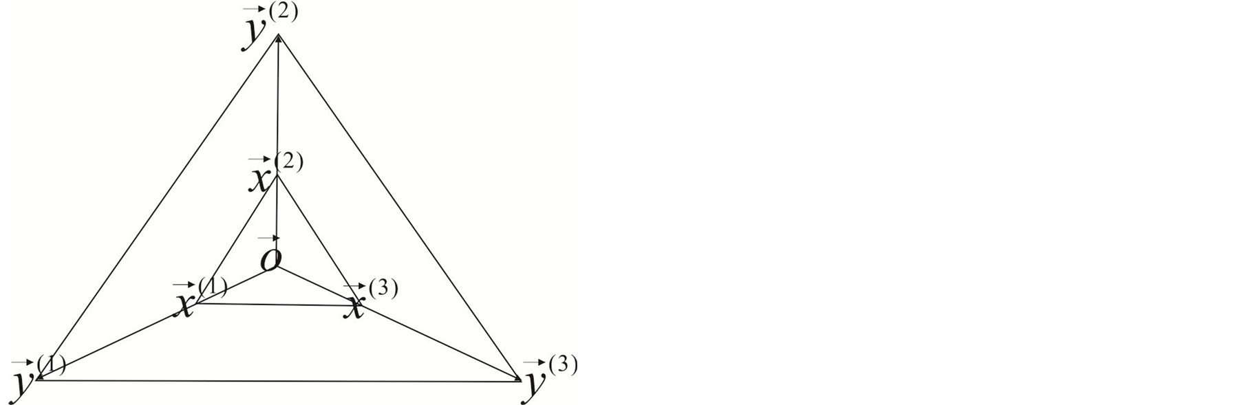
Figure 1. Illustration of a three-parent SPX operator.
4c: Choose two parents randomly from population Pt;
4d: Combine the randomly selected two parents (4c) and  created offspring (4b) to form a population S;
4e: Rank individual of population S, choose the best two individuals;
4f: Replace the chosen two parents (4c) with these two individuals to update Pt.
Step 5: Repeat the above procedure from Step 3 to Step 4 until a certain stop criteria is satisfied.
3. Numerical Example
The performance of the mPRCGA based management model is tested on a hypothetical example considering multiple management periods.
3.1. Description
The example is to deal with the minimization of pumping cost from an unconfined aquifer system and it is assumed that the numbers and locations of the candidate wells are known. This example was previously solved using DDP (Differential Dynamic Programming) by Jones et al. (1987), GA and SA by Wang and Zheng (1998), and HS (Harmony Search algorithm) by Ayvaz (2009). Figure 2 shows the plan view of the aquifer system under consideration.
Groundwater is pumped from an unconfined aquifer with a hydraulic conductivity of 86.4 m/day and specific yield of 0.1. As can be seen from Figure 2, boundary conditions of the aquifer include the Dirichlet boundary at the north and no-flow at the other sides. The distance between land surface and aquifer bottom is 150 m. The flow model is transient; it is assumed that initial hydraulic head value is 100 m everywhere.
3.2. Optimization Model
The total management period is one year, which is divided into four stress periods of 91.25 days each. There are eight candidate pumping wells, and the water demands for each period are 130,000, 145,000, 150,000, and 130,000 m3/day, respectively. The hydraulic head must above zero (bottom) anywhere in the aquifer, and each pumping rates must be in the range of 0 to 30,000 m3/day. The objective function to be minimized is in the form of Equation (2) with T = 4. Note the first two terms in Equation (2) is neglected and Equation (2) is reduced to the last term.
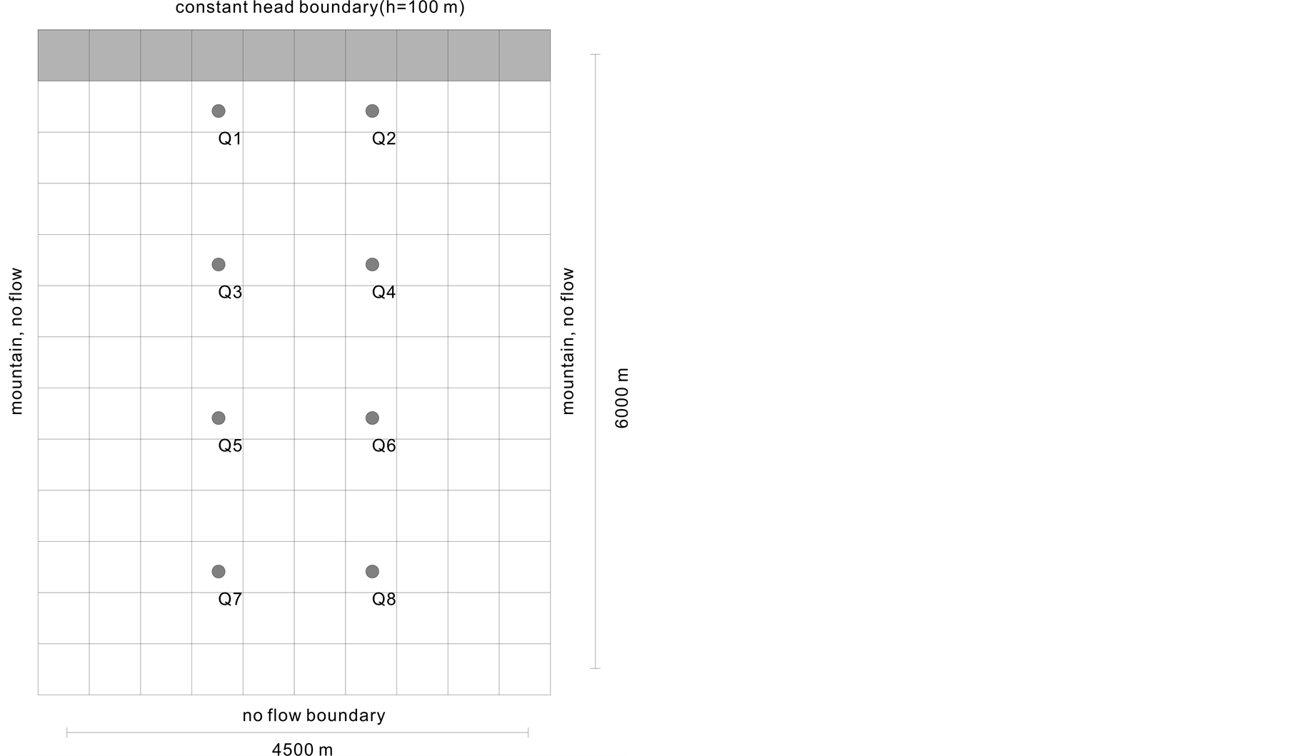
Figure 2. Plan view of unconfined aquifer model.
3.3. Results and Discussion
Using the parameter sets given in Table 1, the optimum pumping rates and total cost has been solved through the proposed mPRCGA based management model. Table 2 summarizes the results of mPRCGA as well as other studies.

Table 2. Comparison of optimum pumping rates and total cost for example 1 by different optimization methods (Unit: m3/d and $).
This shows that the results of mPRCGA are in good agreement with the water demands for each period. Also, pumping rates of wells near the Dirichlet boundary condition are higher than other wells (Q1 = Q2 > Q3 = Q4 > Q5 = Q6 > Q7 = Q8), as expected. The results obtained by mPRCGA also satisfies the requirement of symmetry of aquifer system, this also verify the reliability of MPRCGA.
Furthermore, by comparison of total pumping cost, MPRCGA finds better objective function value (29,539,705 $) than GA (29,779,432 $), SA (29,572,110 $), and HS (29,540,860 $). DDP gives a better result (28,693,336 $), may be due to the stage-wise decomposition of the algorithm. However, the realization of DDP is much more complex. The contrast in pumping rates in 1st period shows that mPRCGA gives closer results to DDP than other methods, and the maximum relative deviation of single well pumping rates is less than 4%. This indicates that proposed mPRCGA is a reliable and effective heuristic optimization method.
Finally, the number of simulations (in Table 2) shows that mPRCGA requires 50,500 simulations, whereas GA, SA, and HS require ~375,000, ~450,000, and 256,615 simulations, respectively.
4. Summary and Conclusions
This study proposes a groundwater management model in which the solution is performed through a combined simulation-optimization model. MODFLOW is used as the simulation model, and in the optimization model mPRCGA approach is proposed. In this approach, a constraint handling technique is presented based on the multi-objective concepts and Pareto dominance is introduced to compute the Pareto intensity number of individual to substitute for the conventional fitness value; meanwhile, RCGA is modified by adopting generalized generation gap model and a modified SPX operator. A hypothetical example is utilized to test the accuracy of mPRCGA. The results indicate that the proposed mPRCGA is an effective method for solving the groundwater management models. Some major conclusions can be drawn as follows:
The proposed mPRCGA can be applied for groundwater management problems, compared with other optimization approaches, mPRCGA can obtain satisfactory results as shown in Table 2;
The parameter sets in mPRCGA, shown in Table 1, is more easily obtained and realized than penalty function methods, this advantage tends to greatly enhance the robustness of algorithm;
To some extent, the modified SPX operator partially overcome the limitation of offspring generation of SPX operator and UNDX operator, together with generalized generation gap model, the modified RCGA may have good ergodic property and high probability to find the global optimum solution.
Acknowledgements
This study was supported by Science and Technology Commission of Shanghai Municipality (No.12231200700).