1. Introduction
Nondestructive testing (NDT) has many industrial applications with increasing use in reliability investigations of materials and components. New and stronger demands on safety, reliability and optimization have made it improper to just detect a flaw or the presence of inferior material properties. The need of quantitative information has given rise to more fundamental approaches to nondestructive evaluation (NDE) with growing emphasis on theoretical modeling of the ultrasonic inspection situation.
In the previous research, we have developed a complete mathematical model of the ultrasonic NDT situation (UTDefect) which has been incorporated into different simulation software (SUNDT and simSUNDT). The development has been ongoing since almost twenty years and has been validated and described in a numerous journal and conference contributions (see e.g. [1] -[3] ). The model includes a general model of an ultrasonic contact probe working as transmitter and/or receiver and the interaction of the ultrasound with the defect. This realistic model offers the possibility of avoiding, or at least reducing, time-consuming and costly experimental work. It can also be useful in the design of inspection routines as it gives an estimate of weather a postulated defect can be detected or not.
The practical situation when ultrasonic NDE is used is in fact an inverse problem, i.e. based on the signals from transmitting and receiving probes an interpretation is performed (see Figure 1). This interpretation is then often based on earlier experiences or by comparing with experimental work or computer simulations. Analytical solutions to the inverse problem have up today only been found for very simple situations and are often based upon a linearization of the inverse problem performed by the Born approximation (an extensive review discussing this is available by Bates et al. [4] ). This linearization limits the applicability since it, at least in principle, restricts the problem to weak penetrable scatterers or low frequencies. Even so this assumption has actually been successfully applied for more complex ultrasonic situations [5] . A slightly different approach, still based on the Born approximation, has been to retrieve a large amount of point source information and address the inversion by various time domain back propagation techniques (Synthetic Aperture Focussing Techniques described in e.g. [6] [7] ). Degtyar et al. [8] introduced an inversion procedure based on a nonlinear least-squares method to determine elastic constants from group or phase velocity data in orthotropic and transversely isotropic materials. Corresponding approach has also been used in order to retrieve viscoelastic material properties based on ultrasonic experimental data (Castaings et al. [9] [10] ).
To investigate its possibility, we approach the inverse problem by applying optimization techniques to our previous general model of the ultrasonic inspection in the present paper. This choice of technique is based on a paper by Björkberg and Kristensson [4] where an optimization technique is successfully used to numerically solve an electromagnetic inverse problem. This problem originates from geophysical prospecting applications and differs from ours in the sense that all components of the scattered field is available by measurements from bore holes in the ground. In ultrasonic NDT situations, only two electric pulses in time, representing the incoming and scattered field, respectively, are the available information from the transmitter and receiver.
The aim of this paper is to investigate if it is possible to numerically solve the inverse problem that occurs in ultrasonic crack detection, by minimizing the mean-square error between the ultrasonic model and corresponding data.
The plan of the present paper is the following. In the first section, we briefly discuss the model of the NDT situation previously presented by Boström and Wirdelius [11] [12] . This includes the probe model, the interaction
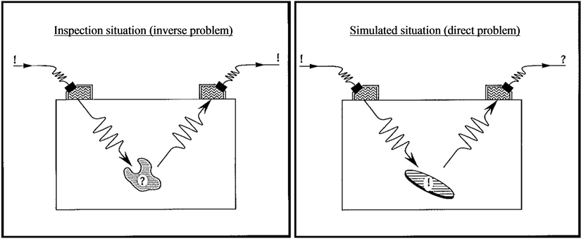
Figure 1. Simulated situation versus inspection situation.
of the probe field with the defect and the reciprocity argument that handles the action of the probe when it is acting as a receiver. The next section presents the optimization technique that is used and is followed by a section with numerical results based on previous sections. Finally, we give some concluding remarks and suggestions for future considerations.
2. Model of the Ultrasonic Inspection
The governing linearized equations for wave propagation in an elastic medium are the equation of motion, Hooke’s law and the strain-displacement relation. If time harmonic conditions are assumed (time factor  is suppressed) these three relations can be combined into the elastodynamic equation of motion governing the displacement field
 (1)
(1)
where

are the compressional and shear wave numbers, respectively ( is the density,
  and
and  are the Lamé constants of the elastic half-space).
The total displacement field is given by the sum of the incident field  and the scattered field
 (2)
(2)
Let us expand the incident field in terms of regular spherical partial vector waves  and the scattered field in corresponding outgoing spherical partial vector waves
 , i.e.
 (3)
(3)
Then it is possible to find a linear relationship between the expansion coefficients for the incident and scattered field and this entity is known as the transition matrix 
 (4)
(4)
All information about the scatterer is contained in its transition matrix and there are various methods of evaluating it. Most common is to use the null-field approach [12] but in our case with a prescribed open penny-shaped crack it is more convenient to use an integral equation method previously described by Boström and Eriksson [13] . The  matrix of a spherical cavity is obtained by separation-of-variables.
We now introduce a coordinate system as in Figure 2 with the  axis normal to the scanning surface and the
  axis chosen so that the probe beam is emitted into the third quadrant of the
  plane with the angle
  with the negative
  axis. In Figure 2, we have introduced
  as the propagation direction and
  is the
  wave polarization direction (with
  and
and ,
,  and
and  as the unit vectors). We choose
  and
and  in order to distinguish between horizontally and vertically polarized shear waves.
In order to model a probe of specific type and angle, the traction vector corresponding to a plane wave of identical type and angle is taken as boundary conditions on the surface of the elastic half-space. Now let the contact probe be characterized by this prescribed traction on the surface of the elastic half-space and assume that this area, corresponding to the acting probe, is elliptic or rectangular.
We then get
 (5)
(5)
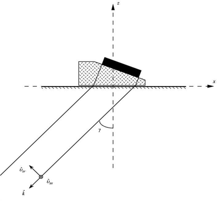
Figure 2. Geometry of the probe with definition of coordinate system and propagation/ polarization directions.
beneath the probe and  elsewhere (A represents the amplitude). The function
  and the constant
  enables reduction of edge effects and varied coupling respectively (for further details see [14] ).
In order to solve this boundary value problem and combine the incident field with the transition matrix formulation, we make following ansatz for the displacement field radiated from the probe
 (6)
(6)
with the plane vector wave functions,  , defined as in Boström et al. [15] , and with the coefficients
  as unknowns. Then the corresponding traction on the surface can be written as
 (7)
(7)
which is identified as a 2D Fourier transform with corresponding inverse transform of the applied traction vector (Equation (5)). This reduces the evaluation of the expansion coefficients to solving a system of equations. In order to incorporate the probe model into the  matrix formulation we have to transform our displacement field from the plane vector waves centred at the contact area into spherical vector wave functions suitably oriented and centred at the defect. This involves a transformation, a translation and a rotation as discussed in Boström and Wirdelius [1] .
The characterization of the probe acting as a transmitter is encapsulated in the expansion coefficients for the incident field  and to evaluate its behaviour as a receiver we use a electromechanical reciprocity argument by Auld [16] and define two elastodynamic states:
 (8)
(8)
(each probe acting with incident power ). Then the change in the electrical response of probe
 , due to the presence of a defect (enclosed by a control surface
 ), is found as
 (9)
(9)
Expanding the two states in spherical vector wave functions and using the Betti identities we end up with the following expression for the electrical signal response
 (10)
(10)
3. Optimization Technique
In the previous section, the theory for the direct problem (the ultrasonic NDT model) has been presented while we in this section introduce the optimization techniques that are used to numerically solve the corresponding inverse problem (see [11] [14] for further details).
The optimization problem is to fit a set of data ,
,  , with a model
 .
.
Let us define the residual function as
 (11)
(11)
where  is a point in parameter space,
  is the coordinate,
  is the data of the
  “sampling” and
  denotes the
  component function of
 . Then the optimization can be stated as a minimization problem (referred to as a nonlinear least-squares problem)
 (12)
(12)
A quadratic model of  around the current point
  is achieved by a two term Taylor expansion
 (13)
(13)
with the Jacobian matrix , with components
  and the second derivate matrix of
  as
as
 (14)
(14)
The next iterate  is then found as the minimizer of Equation (14) by applying Newton’s method (see Dennis and Schnabel [14] ), i.e.
 (15)
(15)
This is a fast local method since it is locally (i.e. near the true minimizer )
)  -quadratically convergent but has the drawback of the necessity of calculating
  which is usually either unavailable or inconvenient to obtain.
Instead of using the quadratic model , we introduce the affine model of
  around the current point
 (16)
(16)
This is an over determined system of linear equations and therefore we cannot expect to find an  that satisfies
 . A logical consequence is then to choose the next iterate
  as the solution to the linear least-squares problem
 (17)
(17)
If  has full rank the solution can be written as
 (18)
(18)
The only difference between the quadratic models  (Newton method) and
  (Gauss-Newton method) is the lack of second order information of
  in the latter which makes it
  -quadratically convergent only if
  (i.e.
(i.e.  linear or
 : a zero-residual problem). If it is a small-residual problem then the convergence will be
  -linear. However, for large-residual problems it may not be locally convergent at all.
In order to enhance the Gauss-Newton method we introduce the singular value decomposition (SVD) of the Jacobian matrix 
 (19)
(19)
where  and
and  are orthogonal matrices. The diagonal elements of
  (i.e. the singular values of
 ) are the nonnegative square roots of the eigenvalues of
  if
if  (or
(or  if
if ) and the columns of
  and
and  are eigenvectors of
  and correspondingly
  if
if .
.
Furthermore we define a pseudoinverse of , the Moore-Penrose inverse, as
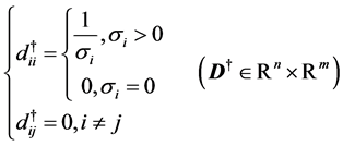

 (20)
(20)
Then the minimizer of Equation (17) is found by (i.e. SVD-Newton iterate)
 (21)
(21)
In order to suppress linear dependence of the column vectors, which will occur in the case of problems that are insensitive to variations of, or a linear combination of, parameters, we introduce the regularized Moore-Penrose inverse as
 (22)
(22)
where the regularizing parameter,  , has the effect of masking off directions in parameter space in which the problem is ill-conditioned.
The previous discussed locally convergent variation of the Newton method has to be supplemented by a global strategy in order to also enable global convergence to the problem. The direction of the Newton step is always a descent direction (if  is limited this includes the Gauss-Newton) but the step may well be too large and therefore not globally convergent.
Given this descent direction,  , and
, and  we try to find
 , with
 , until we get
 (23)
(23)
if also
 (24)
(24)
is satisfied. Then there can be proven that given any direction  such that
 (25)
(25)
there exists  such that any method that generates a sequence
  obeying these three conditions
 , is at each iteration globally convergent. Let us define
  and, if we need to backtrack, use the most current information about
  to model it, and then take the value of ζ that minimizes this model as our next value of
 .
.
Initially we have; ,
,  and
and , which result in the following quadratic model of
 (26)
(26)
then
 (27)
(27)
and  is our new choice of
 .
.
In order to ensure proximity we in the numerical calculations start up with a SVD-Newton step (using Equation (22)) and if this full step does not give an acceptable decrease in the residual we use the above described backtracking line search along this direction.
4. Numerical Results
In this section we present numerical examples of the optimization algorithm developed by Björkberg and Kristensson [11] and here implemented into the elastodynamic problem of defect detection. Our choice of NDEsituation has been the pulse-echo measurement on a elastic half-space with the material assumed to be steel with compression and shear wave speeds 5940 m/s and 3230 m/s (Poison’s ratio ). A major limitation of the numerical optimization is of course the necessity to postulate the defect geometry (i.e. a priori information on the used
  matrix).
We have restricted our optimization to three combinations of defect geometry and scanning probe: spherical cavity (diameter 10 mm) detected with an unangled circular (diameter 10 mm) P probe, open horizontal pennyshaped crack (diameter 10 mm) detected with an unangled circular (diameter 10 mm) P probe and the same crack lying perpendicular to the surface scanned by a 60˚ angled quadratic (side 10 mm) SV probe. All defects are situated at a depth of 60 mm and given a radius of 5 mm and corresponding single frequency C-scans are found in Figures 3(a)-(c)) with individual normalization.
These three ultrasonic inspection situations all contributes with four parameters which we then seek in our optimizations. These four parameters are the  and
and  coordinates, the depth a (of the defect centre) and the defect diameter d. The deviations from the true values are given in percentages and for a and d these percentages are relative the values
  and
and . For the
  and
and  coordinates, however, the percentages are somewhat arbitrarily given relative (−10, −15), (−10, −15) and (70, −10) mm for cases 3A-C, respectively (these are the distances from the defect to the lower left corner of the C-scans in Figures 3(a)-(c)). To identify what information our residual should be based upon we have done parametric studies and these are presented in Figures 4-6. These show that phase information in our case is not useful as a residual which is most obvious when we vary depth or size of the scatterer. The residual is also shown to be more sensitive to the number of frequencies than to the actual number of geometrical samplings points. This effect is revealed in Figure 5 when compared with Figure 4 and is most obvious for the size parameter.
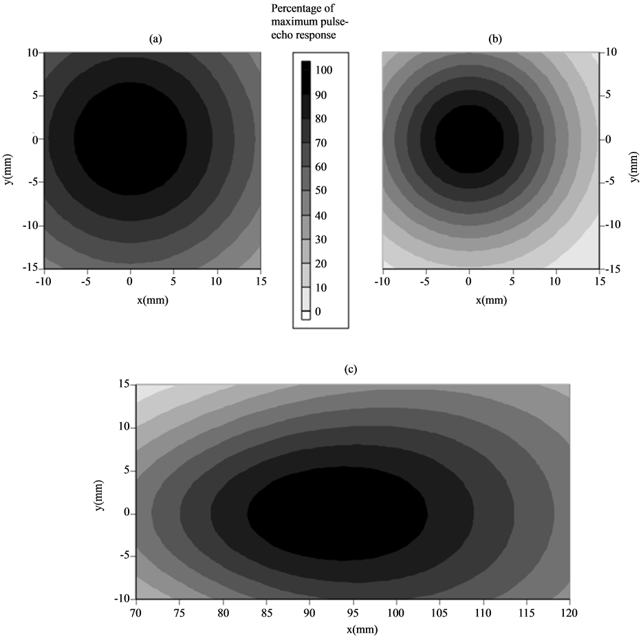
Figure 3. Pulse-echo amplitude as a function of probe position (all probes operating at 1 MHz single frequency): A/ Unangled circular (diameter 10 mm) P probe with a spherical cavity defect (diameter 10 mm) located at the depth 60 mm. B/ Unangled circular (diameter 10 mm) P probe with a penny-shaped crack (diameter 10 mm) located at the depth 60 mm and parallel to the surface. C/60˚ angled quadratic (side 10 mm) SV probe with a penny-shaped crack (diameter 10 mm) located at the depth 60 mm and perpendicular to the surface.
In the expression for the expansion coefficients,  and
and , a double integral has to be evaluated. To avoid a quite computer time-consuming numerical integration (i.e. Gauss-Legendre qudrature), we have chosen to evaluate this with the two-dimensional stationary-phase method (the distance between defect and probe is used as the large parameter). In the far field this have been found to be accurate at least within the main lobe (see [1] ) and in order to avoid what is referred to as an “inverse crime” (see Colton and Kress [17] ), we have also optimized with a “stationary-phase solver” on a integral solution of the direct problem. It is also necessary to suppress the compression part when using an angled SV probe to get the optimization successful.
The time dependence is easy to obtain by an FFT algorithm, but even if the time window is easy to predict and thereby kept small this involves dealing with a waste number of points without any valid information since the response is a pulse in time. Therefore we have chosen to optimize in the frequency domain but with a similar
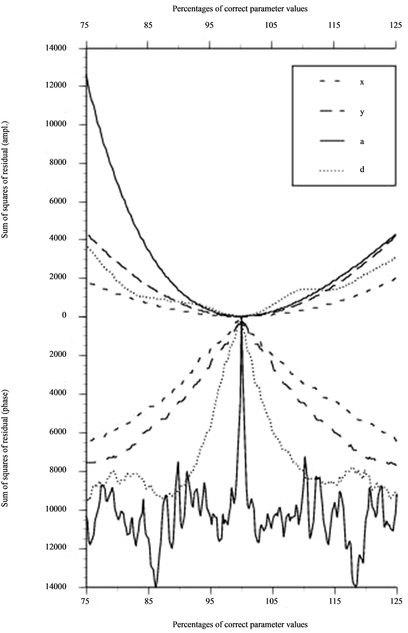
Figure 4. Amplitude residual and phase residual as a function of deviation from correct parameter value for NDE situation 3A. Parameters are: x and y coordinate, the depth a and the diameter d of the defect. Based on information from 12 freq. and 12 × 12 geometrical points (m = 1728).
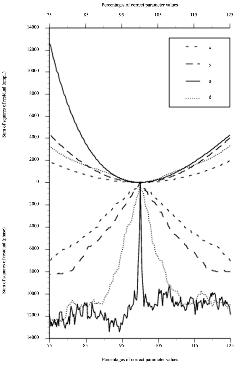
Figure 5. Same as in Figure 4 but based on information from 50 freq. and 6 × 6 geometrical points (m = 1800).
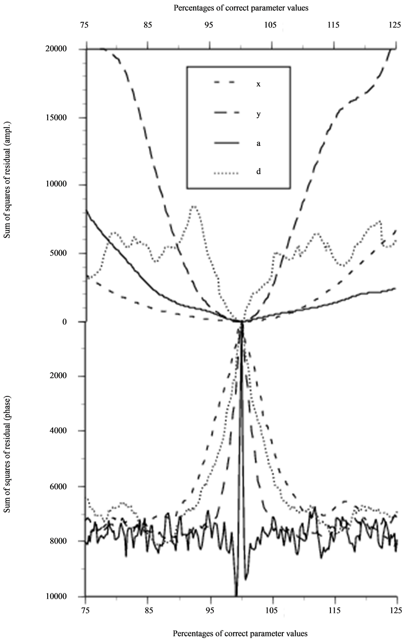
Figure 6. Same as in Figure 4 and Figure 5 but for NDE situation 3B based on information from 10 freq. and 11 × 11 geometrical points (m = 1210).
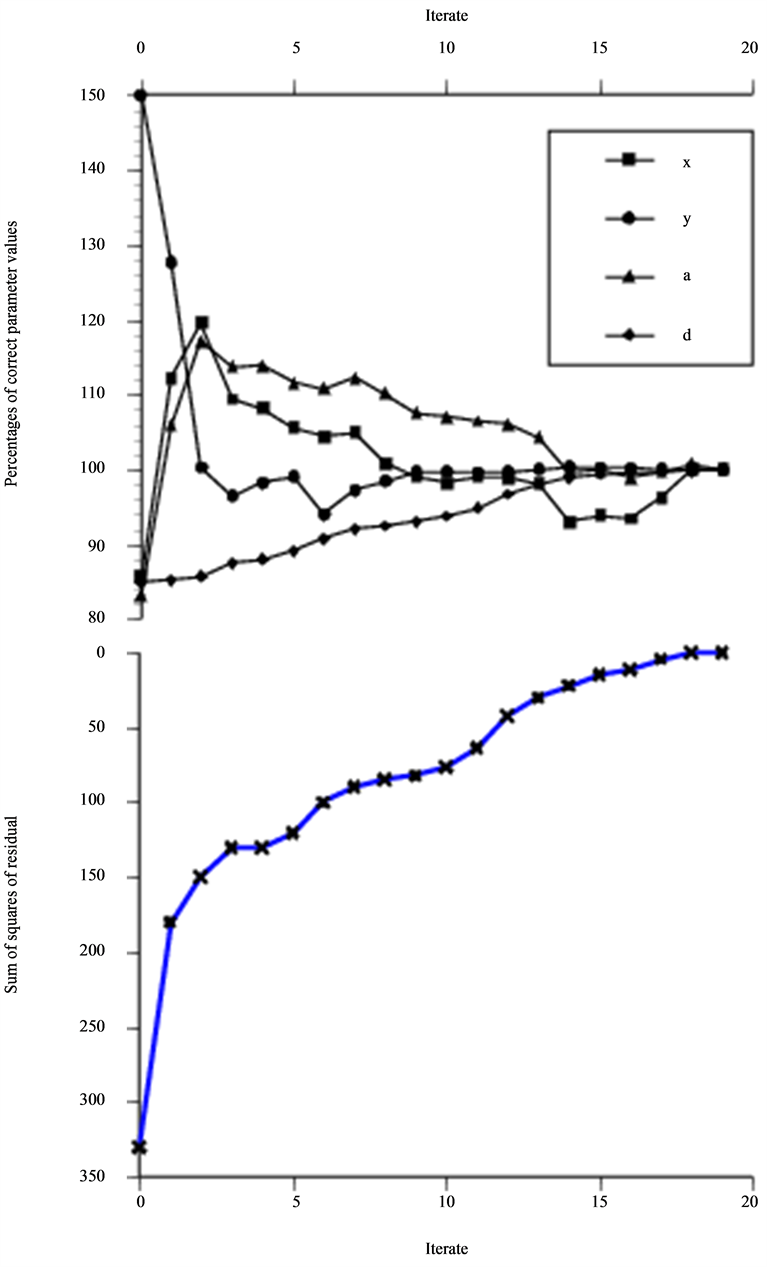
Figure 7. Optimization on situation 3C based on information from 50 freq. and 6 × 6 geometrical points (m = 1800).
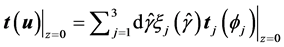
weight function characterizing the probe as that proposed by Boström and Wirdelius [1] . In this model a symmetric sine square function is used as the frequency spectrum and our model of the signal response can therefore be written as
 (28)
(28)
with  as the product of geometrical sampling points and the number of frequencies.
No normalization has been incorporated into the ultrasonic NDT model and therefore the actual residual value is individual in each case. The maximum amplitude of signal response for the three cases shown in Figure 3 varies as  and
and .
.
The parameter that is limiting the optimization is the size and this is also obvious in the parametric study of the penny-shaped crack parallel to the scanned surface. In fact, the number of frequencies had to be increased to 50 (10 frequencies are used in Figure 6) in order to get the optimization to converge. Even then the initial guess had to be within a deviation of 15 percentages in order to converge.
Figures 7-9 shows the result from the optimization of the situation of a 60˚ angled SV probe with a penny-shaped crack perpendicular to the surface. In Figure 7 the initial guess of crack diameter is 85% of the
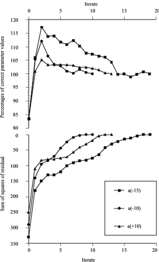
Figure 8. The depth variation when optimization is performed as in Figure 7 and for three initial guess of defect diameter.
correct value and all the parameters convergence rate is presented in the figure while we have chosen to present the diameter and depth convergence rate as a function of initial guess of diameter in Figure 8 and Figure 9, respectively. This is due to the fact that these two parameters are not independent of each other. The over-estimation of the depth at second iterate found in Figure 8 is as seen strongly dependent on the initial guess of diameter and critical in terms of convergence. The two major stopping criteria of the optimization are the distance between two steps and sufficient decrease of the residual.
In Figure 10, we present the optimization on the same NDT situation using an asymptotic probe model on data achieved by the corresponding integral solution. This reduce the convergence from being q-quadratical to being q-linear and the number of iterates increases from 20 to 25 before the stopping criterion of step size ends the optimization. At the minimum all parameters are within 1% deviation from the values representing the “true” minimizer, except for the x parameter that ends at 96% of its corresponding value.
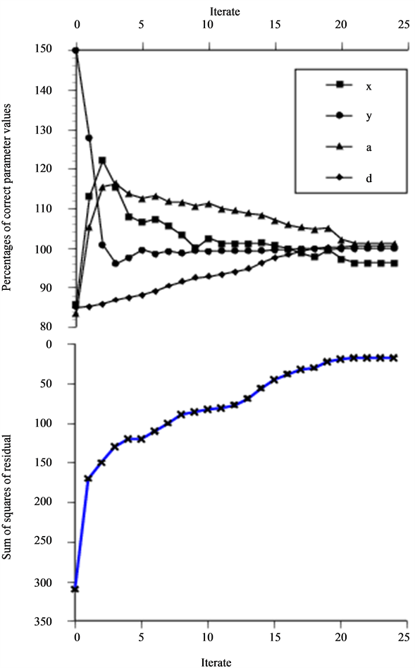
Figure 10. Optimization as in Figure 7, performed with asympt. probe model on data generated by corresponding integral solution (non-zero residual probl.).
Figure 11 present the result of the optimization on the situation of an unangled P probe with a penny-shaped crack parallel to the scanning surface. The problem with overestimation of the depth parameter at the second iteratation is also present for this situation. Even though this effect is more pronounced in this case, the true minimizer is already found at the 10:th iterate.

Figure 11. Optimization on situation 3B based on information from 50 freq. and 6 × 6 geometrical points (m = 1800).
In Figures 12-15, the type of defect is altered to a spherical cavity and scanned by an unangled P probe. For this situation the dependence between depth and diameter are even more obvious since the maximum signal response is dependent on the distance represented by the difference between these two. The asymptotic probe model is used for data in Figure 12 while the numerical integrated solution is data in Figures 13-15. The non-zero residual problem in Figures 13-15 reduces the rate of convergence in terms of iteration as expected but the optimization actually becomes more insensitive to deviations from the “true” value in the initial guess of the size. At the minimum a cavity two percentages larger and oriented two percentages less in depth than that used to generate the data is found.
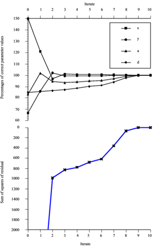
Figure 12. Optimization on situation 3A based on information from 50 freq. and 6 × 6 geometrical points (m = 1800).
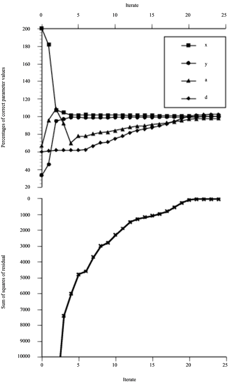
Figure 13. Optimization as in Figure 12, performed with asympt. probe model generated by corresponding integral solution (non-zero residual probl.).
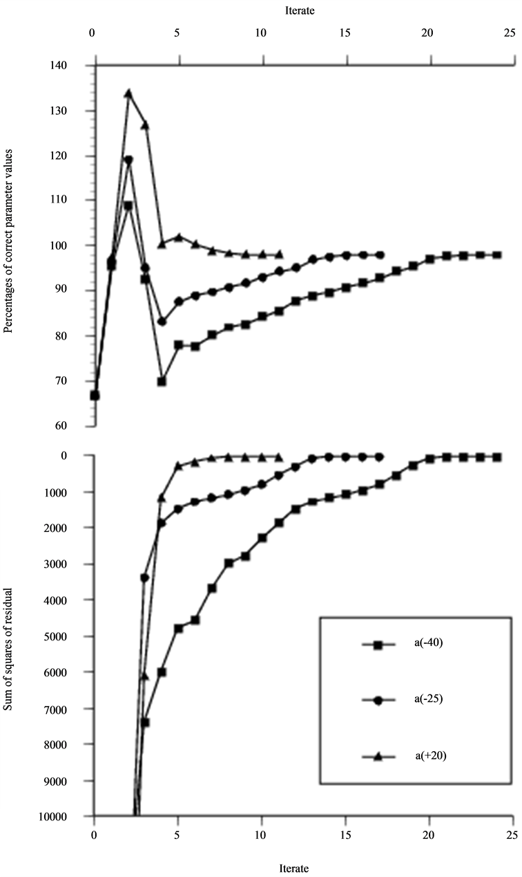
Figure 14. The depth variation when optimization is performed as in Figure 13 and for three initial guess of defect diameter.
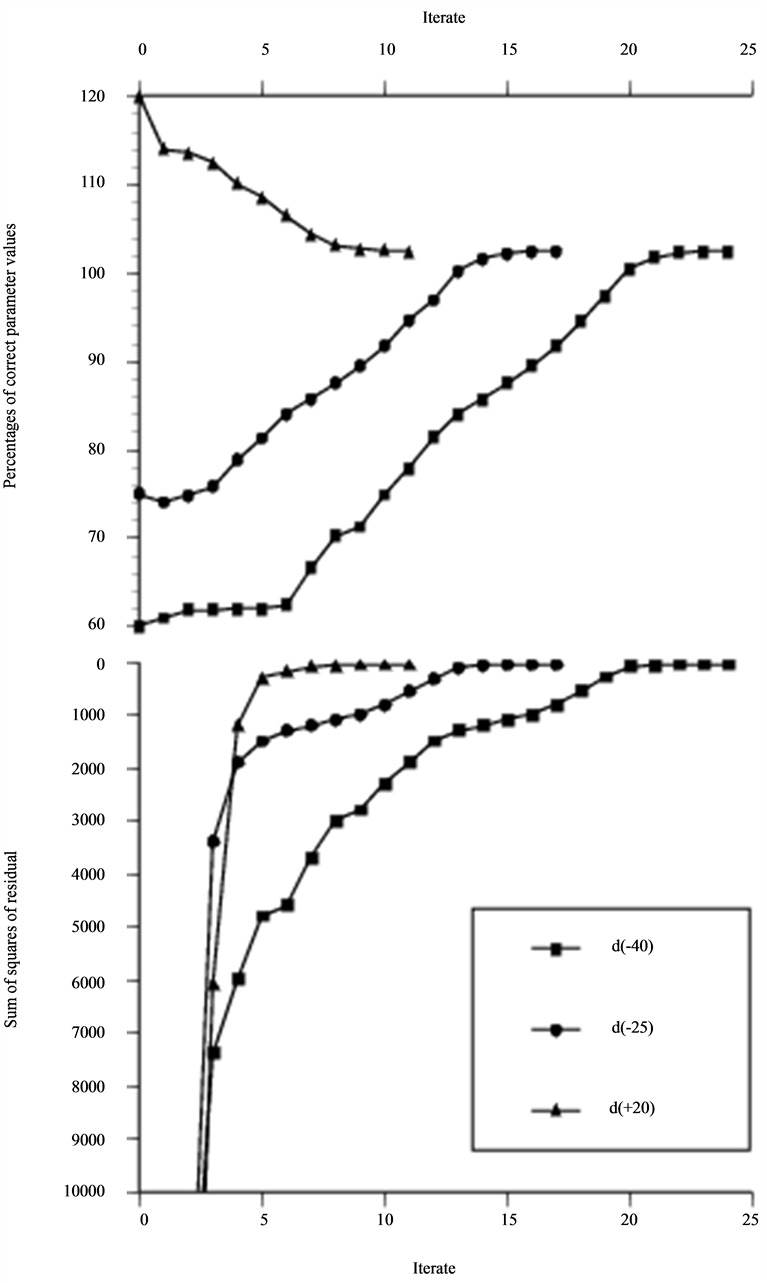
Figure 15. The diameter variation when optimization is performed as in Figure 13 and Figure 14.
5. Concluding Remarks
In the preceding sections, we have studied a numerical inverse solution to the non-destructive testing situation. The method we have used to achieve this has been the application of an optimization technique on a model of the ultrasonic inspection situation. If the inverse algorithm, described in previous sections, is to be used together with experimental NDT data a more general T matrix has to be implemented. Such as the T matrix for an elliptic or rectangular crack, oriented by three Euler angles, increases the number of parameters to eight which call for improvement of the convergence. One conclusion that can be made from the numerical section is that there is a distinct difference between global parameters compared with local (i.e. 3A/3B: a and d, 3C: x, a and d), in terms of convergence.