A Receiver Model for Ultrasonic Ray Tracing in an Inhomogeneous Anisotropic Weld ()
1. Introduction
In-service inspection of components that includes welds in austenitic stainless steel and Inconel metal has revealed systematic faults that are due to unpredictable paths of the ultrasound in the welded material. These welds exhibit not only highly anisotropic behavior but also involve inhomogeneous ultrasonic properties. This is caused by the solidification process and the orientation of the dendrites (i.e. large grain structures) is governed by the temperature gradient in the cooling process.
Modeling of ultrasonic non-destructive testing (NDT) is important and helpful e.g. in predicting the response of an NDT inspection, correctly analyzing output data or acquiring a medium’s mechanical properties. Many endeavors have been made to simulate this process. Among them, some special efforts are made to ultrasound propagation through an anisotropic weld [1] -[7] . When ultrasonic NDT is performed on a weld with strong anisotropy, special phenomena may occur compared to same inspection conducted on an isotropic medium. For example, the group velocity does not necessarily have the same propagating direction or amplitude as the phase velocity. This will make ultrasound beams propagate in an unexpected or unpredictable way through a weld.
This paper is a part of an initiative to develop a methodology that estimates grains’ orientations in an anisotropic weld by using ultrasonic information in an inverse scheme. Well defined anisotropy in the simulated volume is prerequisite in order to make simulations of the forward problem, i.e. ultrasonic inspection of an anisotropic weld. The framework of such an initiative consists of a weld model, a forward 2D ray tracing model, experiments and an inverse problem solver. The latter justifies the limitations in the simplified model presented in this paper (e.g. 2D model, no mode conversion and ray tracing). The assumption of the weld being two dimensional and transversely isotropic is often used [8] -[12] and has recently also been experimentally validated [13] . Furthermore, the grain orientation is believed to be an essential factor that affects the propagation of ultrasound. In most simulation cases, a simple weld model is created by studying the macrograph of an austenitic weld. Different algorithms are then utilized to simulate the propagation of ultrasound through weld models. There also exist other methodologies to deduce anisotropic weld models that are not based on information retrieved from macrographs from reproduced welds. Gueudre et al. [14] have created a model by considering the welding process. In their models, the grain’s orientation at different positions is decided by several parameters such as the chamfer geometry, the number of passes and the diameter of electrodes.
Another 2D ray tracing model was recently validated by using EFIT calculations [15] with very good agreement. In simulating the propagation of ultrasound through the weld model, the ultrasonic beam is approximated for high frequencies as a ray. The direction of the ultrasonic energy is continuously followed. Transmission and reflection are considered on the fusion lines between the base material and the weld, as well as on the boundaries between the sub regions in the weld. In the simulation, no mode conversion between the P wave and the SV wave is considered. This can be experimentally assessed by gating out the received information in thoroughly chosen time window. As a consequence, only the wave with the same mode is traced from the transmitter to the receiver.
In the present paper, a receiver model is presented, which is a continuation of a previously developed forward ray tracing model [16] . For the modeling of a receiver in an ultrasonic NDT system, Auld’s electromechanical reciprocity principle [17] [18] is the most well-known approach. In most cases, it is applied to simulate the detection of a diffracted signal from a scatterer in a medium [19] -[22] . The reciprocity principle is employed to model the detection of the ultrasonic transmitted signal in the 2D ray tracing program. There are seven sections in this paper. The second section is a brief retrospect of the weld model and the forward ray tracing model. It is followed by a discussion of the receiver model. Simulations and validations of the receiver model are introduced in Sections 4 to 6. Discussions and concluding remarks are presented in Section 7.
2. A Retrospect of the Established 2D Ray Tracing Model
The forward model is composed of four main elements: a weld model, a transmitter model, a 2D ray tracing algorithm and a receiver model. In a previous paper [16] , the first three models have been presented. A brief description is repeated here.
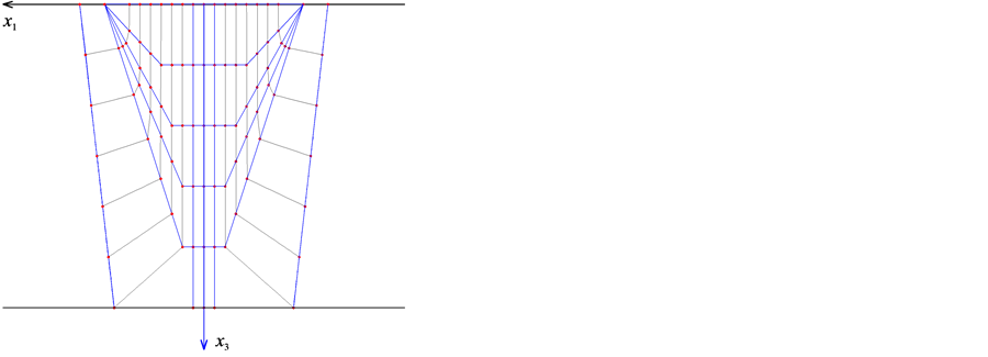
The weld model is established by studying the crystalline structure of a V-butt weld. The prototype is a weld specimen provided by Swedish Qualification Center (SQC) and defined as weld B27 in [17] . Following the process of creating a weld model introduced in the previous paper and based on the macrostructure identified in Figure 1(a) the weld model is defined as shown in Figure 1(b). There are about eighty sub-regions in it, which have their own particular grain orientations. Each sub-region is considered homogeneous, lossless and transversely isotropic. For the weld model used in this paper, the grains’ elastic constants are ,
,  ,
,  ,
,  ,
,  and
and  (with the axis of symmetry in the local
  -direction) and the density is
  [17] . The base material outside the weld is modeled as conventional stainless steel and is prescribed to be isotropic (Lamé constants
 ,
,  and density
 ). The dimension of the weld is as follows. The upper width is assumed to be 18 mm, and the lower width is 13 mm. The height is supposed to be 22 mm. For the convenience of the ray tracing simulations, the curved boundaries in the original weld model is further replaced by straight lines, which is shown in Figure 1(c).
The model of the transmitter is created from a truncated traction distribution representing the pressure produced by the probe on the surface of the component [16] . The traction distribution is correlated to a presumed plane wave propagating in a half-space with prescribe direction. Taking a plane  wave as an example, in the frequency domain, it can be described by the following expression,
 (1)
(1)
where  is the amplitude of the wave;
  is the angle between the propagation direction and the
  axis, and
  is thewave number. A diagram describing this assumption is shown in Figure 2.
A truncation of the corresponding traction distribution along the upper surface of the half-space is performed, which provides
 (2)
(2)
 (a)
(a) (b)
(b) (c)
(c)
Figure 1. A weld model is generated by studying the macrograph of a typical weld.

Figure 2. The transmitter model is generated from a presumed plane wave propagating in an isotropic half-space.
where  is the shear modulus and
  is the wave number of the
  wave.
wave.
If Fourier transform in  is fulfilled, the above truncated traction distribution is
 (3)
(3)
In this expression,  and
and 
Hence, Equation (3) is taken as the model of the ultrasonic transmitter.
A simple 2D ray tracing algorithm has also been developed. The ray direction, which is also the ultrasonic energy direction, is derived from the relationship between the phase velocity and the energy velocity (the energy velocity must always be normal to the slowness surface). Since the group velocity and the energy velocity are identical for acoustic waves in a lossless medium, an expression can be utilized to calculate the energy velocity [23] ,
 (4)
(4)
with  and
and  as the components of the wave vector in
  and
and  directions [16] . Transmission and reflection on the fusion lines between the weld and the base material, as well as on the boundaries between different sub-regions in the weld model are considered, which produce both the transmitted ray direction and the relative amplitude. Mode conversion is neglected in this 2D ray tracing model, which means that only waves of a single type are followed continuously. If there is no transmitted body wave generated, the ray tracing algorithm will stop.
3. The Receiver Model
In the modeling process, the ultrasonic testing is assumed to be performed with a transmitter-receiver structure of pitch-catch configuration. According to Auld’s reciprocity principle, the response of the receiver model can be expressed by the change of the electrical transmission coefficient between two states that correspond to the situations with or without a scatterer. Hence, the response of the ultrasonic receiver model can be calculated as
 (5)
(5)
here,  is the angular frequency and
  is the probe electrical power.
  denotes the border of a closed integration contour surrounding the scatterer,
  denotes the displacement vector, and
  is the traction. Subscripts 1 and 2 indicate that the field is linked to two different states, 1 and 2. It is the difference between these two different states that produces the change in the electrical transmission coefficient. Auld’s reciprocity argument is only valid for a loss-free medium (i.e. no viscous damping) which is modeled in this case. The found deviations between experimental and simulated results presented in next chapter could partly be explained by this diversity.
For the receiver model in this paper, state 1 is chosen as the actual testing situation. As shown in the left part of Figure 3, in this state the transmitter works in the presences of the reflecting back wall and the weld. The “scatterer” in Auld’s formalism [18] then consists of both the weld and the lower back surface. The transmitter is located at positions along the negative  axis and outside the weld. In state 2, the scatterer, defined above, is absent. The receiver acting as a transmitter then works over a homogeneous half-space with the same elastic properties as the base material. In addition, the transmitter functions along the positive
  axis and outside the weld. When performing calculations according to Equation (5), the integration contour is selected as the dotted lines in Figure 3. Thus, the whole scatterer is enclosed by the integration contour and the main task in simulating the

Figure 3. Illustrations of state 1 and 2 in the reciprocity model.
received signal is to determine the displacement  and the traction
  along the integration contour in these two states.
Since the weld’s upper border  is assumed to be traction free in both states, this part of the integration gives no contribution to the calculation. In addition, the borders
  and
and  are traction free in state 1 because the lower half-space is considered to be a vacuum. While in state 2, since there is no scatterer, the borders of
  and
and  are not treated as traction free as they are part of the infinite halfspace. In addition, fields in both states are calculated in the isotropic media on the boundaries
 ,
,  ,
,  and
and .
.
On the side of incidence, two different cases are considered in state 1. The first case is that ultrasound impinges directly on the boundary  and propagates through the weld. The second case is that the ultrasound first impinges boundary on the
 , and then the reflected wave impinges on boundary
  and propagates further. Similarly, on the other side of the weld, the transmitted wave may first reflect on the boundary
  and then terminate at the upper border. Or it may run directly to the upper border. Therefore, in state 1, reflected fields on the boundaries
  and
and  are considered.
Let us assume a  wave being reflected on
  as an example (the
  wave reflection on
  and the SV wave reflection can be dealt in a similar way). The incident plane
  wave is then propagating within the isotropic part and can be defined by the following expression,
 (6)
(6)
As in Equation (1), A is the displacement amplitude of the  wave.
wave.  and
and  are wave numbers in the
  and
and  directions, respectively. The wave number
  satisfies
 . The total displacement field (the reflected SV wave is neglected) becomes
 (7)
(7)
where  is the reflection coefficient given by literature [12]
  .
.
Reflected fields on the boundary  are not taken into account in the model because it is believed to give only a small contribution to the total field. As mentioned above in the forward ray tracing program, no mode conversion is considered in the calculations. The traction components on the boundary are given by
 , where
  is the component of the inward directed normal
  of the boundary. The stress
  is determined by Hooke’s law
 . Here,
  is the stiffness matrix. The strain
  is related to the displacement by
 . In these expressions, Einstein’s summation convention is used.
4. Experimental Setup
Since neither mode conversion, viscous damping or any coarseness of the weld are included in the model at this stage, the intention with the validation is to identify necessary modifications in the experimental procedure or essential limitations in selecting weld, when the inverse problem in a later stage is to be addressed. The validation only intends to qualitatively validate the variation in anisotropic properties in the welding direction, in an ultrasonic pitch-catch perspective.
The experimental part of this project was performed by the Swedish Qualification Center (SQC) according to instruction (i.e. procedure) developed in collaboration with Chalmers. The purpose to collect data from real inspection objects with material structure defined by the welding specifications is to compare experimental data with theoretically calculated values. The three-dimensional welded volume is piecewise modeled by two dimensional line scans with variation of the predefined anisotropic orientation in each individual scan.
Collection of data has been performed by keeping one probe on a fixed distance from the weld centre line and moving the receiving probe perpendicular to the weld in line with the other probe (see Figure 4). This has been repeated along the weld with an increment of 4 mm. Further details of used equipment, welding specifications and information of the procedure to collect experimental are specified in [17] .
5. Simulations
The output of the ultrasonic NDT system, expressed by the change in the electrical transmission coefficient, is calculated according to Equation (5), but in a discrete form on each boundary. The expression in Equation (5) is approximated by
 (8)
(8)
In the calculations, 100 discrete points are preset evenly along the fusion lines  and
and , with an interval of
 . The number of integration points on
  and
and  is determined by
 (9)
(9)
where  is the horizontal distance between the lower left corner (or the right corner) of the weld and the assumed furthest scanned position. In the simulation, the scan is supposed to cover from 10 mm to 108 mm along the upper surface of the base material, out of the weld. Therefore,
  is adopted and then
 . In order to simulate the main lobe generated by a real ultrasonic transmitter, seven rays are adopted in each simulation. The simulation result of the receiver model is the superposition of the contributions from these rays. These seven rays are distributed evenly between
  from the transmitter’s nominal angle (i.e. prescribed angle [21] ). To determine the parameter
  in the simulation, an expression in Krautkrämer and Krautkrämer [24]
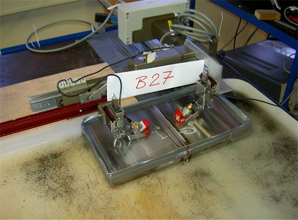
Figure 4. A picture of the experimental setup with the transmitter and receiver in a tandem configuration.
is referred to. It says that, for a circular piston oscillator, the divergence of the beam  is approximately
 (10)
(10)
In this expression,  is a factor whose value is supplied in a reference table to suit different sizes of the main lobe.
  is the ratio of the sound pressure on the edge to the maximum,
  is the wavelength, and
  is the aperture of the probe.
In this paper’s calculation,  adopts the value of
 . This corresponds to a main lobe whose sound pressure on the edge is about 84% of the maximum, almost 1.5 dB which correlates with the ray assumption in the model. For a P wave probe of 2.25 MHz, the wavelength is
 . In the 2D transmitter model, the aperture of the transmitter is
  and the calculation from Equation (10) gives
 . Similarly, for an SV wave probe of 1 MHz,
 . Based on these values
  is chosen. Since the plane wave assumption is made in the modeling, the calculation of the displacement amplitude of a ray in the transmitter model is based on the far-field amplitude information at a fixed distance from the transmitter. Moreover, when a ray impinges on a boundary, only points lying in an area with a length of l around the intersection by the ray and the boundary is considered influenced by the ray. Points outside this area are not affected by the ray. Therefore, fields are not calculated for these points. Experiences made from the simulations revealed that
  was a good choice. To simulate different sections in a C-scan display, a different random variation with a maximum of ±5% is introduced in the grain orientations in each run of the calculation. The intention is to validate the degree of variation along the welding direction and qualitatively compare with the C-scan plots achieved from the experiments. Grains with an orientation of 90˚ to the
  axis (mostly in the center of a weld, as shown in Figure 1(c)) are free from this random change because they are believed to be close to the actual situation.
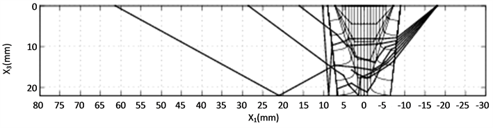
Two different groups of simulations are performed for the same weld model, one for the  wave and another for the SV wave. In each group, three different cases are simulated. Parameters for each case are listed in Table 1 with the transmitter positions defined in Figure 5. The experiments were set up under the same conditions as listed in Table 1 and executed at SQC. Simulation results, as well as the corresponding experimental results are shown in Figures 6-17. Figure 6, Figure 8 and Figure 10 are simulation results for the P wave. They correspond to a transmitter position of −18 mm, −33 mm and −67 mm (along the x1 axis), respectively. For the SV wave, Figure 6, Figure 12 and Figure 14 are the simulation results of three different transmitter positions of −18 mm, −24 mm and −36 mm, respectively. Transmitter positions in the model’s coordinate system are shown in Figure 3. In each figure, subplot (a) is the plot of one of the ray tracing runs. There are totally nine runs because of the adoption of nine groups of randomness in the grain orientations. Here only the last group of the simulation results among the nine runs is displayed for each simulation shown in subplot (a). Subplot (b) is the output of the receiver model corresponding to the different randomness taken in grain orientations in the simulations. Subplot (c) is also the output of the receiver model, but depicted in a surface plot (i.e. a simulated C-scan). The
  axis in this subplot indicates different sections corresponding to a C-scan, and the subplot (c) shows a fluctuation in the signal response due to the randomly variation in grain direction in each individual line scan. To facilitate the comparison, the simulation results of the
  wave receiver model in Figure 6, Figure 8 and Figure 10 are first normalized with the maximum in Figure 6(b), and then transformed into decibel from 0 to −20 dB. The figures of the SV wave calculation are dealt with in a similar manner, but normalized with the maximum in Figure 12(b).
6. Validations
Experimental results of ultrasonic C-scan are displayed in Figure 7, Figure 9 and Figure 11 for the  wave.
wave.

Table 1. Experimental parameters on a specific weld.

Figure 5. The relationship of the coordinate systems used in the simulation and the experiment.
 (a)
(a) (b)
(b) (c)
(c)
Figure 6. Simulation result of the P wave (probe position is −18 mm). (a) Ray tracing plot; (b) Receiver model output 1; (c) Receiver model output 2.
Figure 13, Figure 15 and Figure 17 are experimental results of the SV wave. In the experiments, a new coordinate system is adopted so as to facilitate the operations, which is shown in Figure 5. Obviously, this is different from the coordinate system used in the model shown in Figure 3. In each run, the distance  of the transmitter from the center of the weld is first determined. Then, the position of the transmitter is taken as the origin. The receiver scans a certain distance
  from the transmitter, in the negative direction. This can be observed in
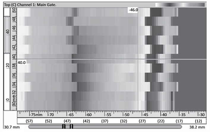
Figure 7. Experimental result of the P wave (probe position is −18 mm).
 (a)
(a) (b)
(b) (c)
(c)
Figure 8. Experimental result of the P wave (probe position is −33 mm). (a) Ray tracing plot; (b) Receiver model output 1; (c) Receiver model output 2.

Figure 9. Experimental result of the P wave (probe position is −33 mm).
 (a)
(a) (b)
(b) (c)
(c)
Figure 10. Simulation result of the P wave (probe position is −67 mm). (a) Ray tracing plot; (b) Receiver model output 1; (c) Receiver model output 2.
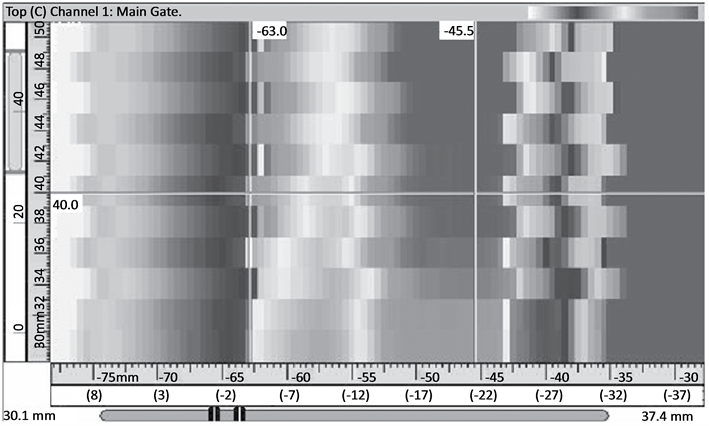
Figure 11. Experimental result of the P wave (probe position is −67 mm).
 (a)
(a)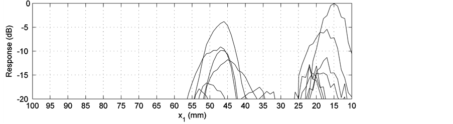 (b)
(b) (c)
(c)
Figure 12. Simulation result of the SV wave (probe position is −18 mm). (a) Ray tracing plot; (b) Receiver model output 1; (c) Receiver model output 2.

Figure 13. Experimental result of the SV wave (probe position is −18 mm).
 (a)
(a)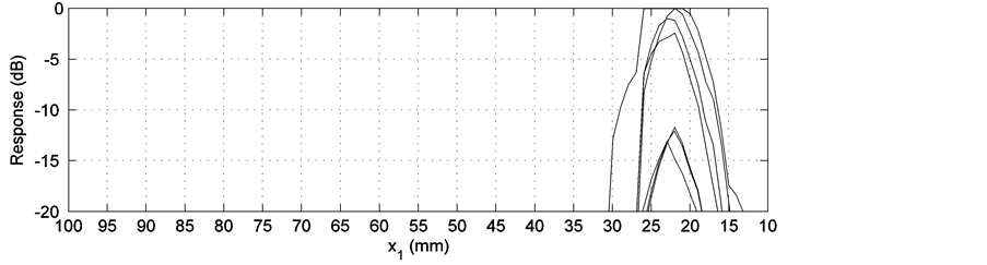 (b)
(b) (c)
(c)
Figure 14. Simulation result of the SV wave (probe position is −24 mm). (a) Ray tracing plot; (b) Receiver model output 1; (c) Receiver model output 2.

Figure 15. Experimental result of the SV wave (probe position is −24 mm).
 (a)
(a)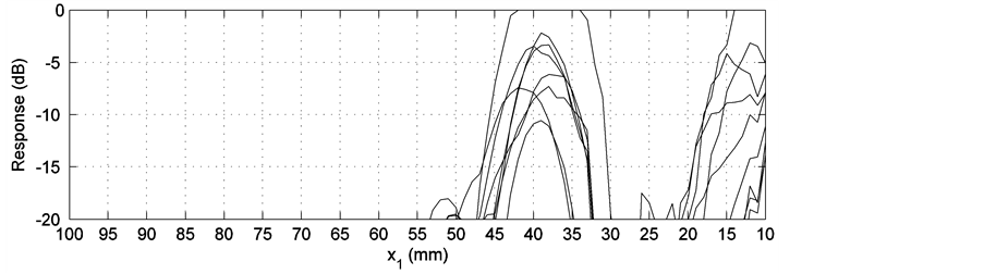 (b)
(b) (c)
(c)
Figure 16. Simulation result of the SV wave (probe position is −36 mm). (a) Ray tracing plot; (b) Receiver model output 1; (c) Receiver model output 2.

Figure 17. Experimental result of the SV wave (probe position is −36 mm).
each figure of the experimental result. The scales of the abscissa on the first line are all negative, from about −30 mm to about −80 mm. For the sake of making a better comparison between the simulation results and the experimental outputs, a coordinate transformation is executed as a post processing. With this coordinate transformation, the coordinate of the receiver is switched to be associated with the weld center, rather than the transmitter. This is realized by , which is illustrated in Figure 5. After the transformation, a new abscissa whose scales are in parentheses is arranged in each figure of the experimental output, under the original abscissa. The experimental data are evaluated with the software UltraVision and displayed in gray palette. This causes the loss of color information. Therefore, an approximate peak position is labeled in each experimental result as a remedy.
When considering the simulation results, it is observed from the subplots (a) that the P wave is less affected by the weld than the SV wave is. For the P wave, all rays can reach the upper surface of the weld model, while some of the SV rays terminate in the weld without further transmission. In addition, some of the SV rays behave irregularly when propagating through the weld model. This phenomenon implies that SV waves are more sensitive to the grains’ crystal orientations, which coincides with common knowledge of the SV wave propagation in an anisotropic medium. On the other hand, this indicates that the weld model has more influence on the SV wave propagation than on corresponding P wave. Therefore, the partition of the weld, as well as the setup of the boundaries between sub-regions is essential for a successful simulation, especially for the SV wave. In addition, mode conversion is not considered in the modeling, which also possibly makes the number of transmitted SV waves too few.
The receiver model presents the distribution of the signal in subplots (b) and (c). A simulated C-scan plot is implemented by the adoption of randomness in the modeled grain orientations. It is noticed that the distribution of the receiver model’s output does not agree with that of the ray tracing plot perfectly. In Figure 6(a), rays occupy the area almost from 30 mm to 100 mm along the upper boundary, while in Figure 6(b) and Figure 6(c), the main peak appears approximately from 37 mm to 52 mm. In Figure 8(a), rays are distributed over the area between 22 mm and 80 mm. But in Figure 8(b) and Figure 8(c), double peaks cover the area between 20 mm and 37 mm. Similar situations also occur in Figure 12 and Figure 16. Good agreement between the ray tracing plot and the receiver model output can only be observed in Figure 10 and Figure 14. In Figure 10(a), rays are terminated between 10 mm and 30 mm. In the corresponding receiver model output, a similar result is achieved. In Figure 14, the only two transmitted rays stop around 27 mm. The receiver model output covers approximately the same place. This phenomenon is believed to be caused by the application of the reciprocity principle. According to the reciprocity relationship, the modeled receiver is the same as the modeled transmitter. Thus, for a 60˚ transmitter, the same type of receiver is supposed. Consequently, only the waves propagating around this angle contributes to the receiver’s main output.
When considering the experimental outputs, it is found that since the scans only cover an interval of 20 mm (from 30 mm to 50 mm) along the weld, marked difference among the sections of a C-scan cannot be noticed for the P wave results. But for the SV wave results, difference among the sections of a C-scan can be observed, e.g. in Figure 13 and Figure 15. In evaluating the P wave data, detailed analyses are always required to discern the true signal from the one caused by mode conversion because the signal strength caused by mode conversion is usually much stronger. This is clarified in Figure 7, Figure 9 and Figure 11, in which the dark areas on the rightmost side are believed to be caused by mode conversion. In addition, in Figure 11, only the left cursor indicates the requested peak signal position. The right cursor is an indication of the mode conversion.
If the receiver model’s output 2 and the C-scan plot of the experimental result are compared, the result is not very satisfying. Even if only the maximum response position is considered, there is a difference between the simulation result and the experimental result. For the P wave experiments, in Figure 6(c), the maximum of the receiver model output is between 40 mm and 50 mm. However, the experimental result presents the maximum around 28 mm in the C-scan display. If Figure 8(c) and Figure 9 are compared, different peak forms can be noted though the areas of maximal signal overlap. Figure 10(b) displays a tendency of having the maximal signal in the weld, which is shown in Figure 11, while quantitative information is missed. This is caused by the limitation of the receiver model, which always starts scans from 10 mm. For the SV wave experiments, similar disparity can be located also. For example in Figure 13, the experiment result indicates clearly that the maximal output is distributed in the area from 26 mm to 33 mm, while in the simulation result of the receiver model, this tendency is quite vague. In Figure 14(c), only some sections display the same distribution area of the maximal signal as in Figure 15. The differences between Figure 16(c) and Figure 17 can partially be attributed to the imperfectness of the weld model and the ray tracing model. Another possibility is the influence of mode conversion that is mentioned above. In the modeling and simulations, mode conversion is not included. In the experiments, the recorded result is a comprehensive action of all the factors that also includes effects such as mode conversion. This could to some extent be filtered out by thorough time gating of the received signal.
7. Concluding Remarks
A receiver model for a 2D ultrasonic ray tracing program is proposed in this paper. It is based on Auld’s electromechanical reciprocity principle. Two different states are employed in the calculation. The first state represents the actual testing situation. The “scatterer” is then present and the transmitter works at the same position as in the actual measurement. For the second state, no “scatterer” is present and the transmitting probe is positioned on the other side of the weld (receiving side). Numerical calculations are performed for both P and SV waves. In each case, three different transmitter positions are used. The distribution of the detected signal then is presented by the receiver model. Simulation results are compared with the C-scan plots from the experiments. In some of these cases there are obvious differentiations. This involves a number of possibilities due to deviations between the idealized mathematical model of the NDT inspection situation and the actual experimental data collected by conventional equipment in an industrial environment. Beside the previous mentioned exclusion of viscous damping in the model also the simplification of the texture in the weld could be part of the explanation. Another plausible cause could be inaccuracies in the collection procedure of experimental data (described in [17] ). The latter also indicates on how essential the time-gating procedure is when, as in this case, mode conversion is excluded in the model.
A point achieved from the validating process and the comparison is that the simulation presents the maximum received signal at a point, while the experiments present the maximum output over an area. Hence, the resolution of the experimental results is vital to the evaluation of the later inversion calculation. How to obtain a reliable result from the experiments and then apply it to the comparison with the forward simulation result is a new challenge.
Acknowledgements
This project is financed by the Swedish Qualification Center (SQC). Kjell Högberg, Gunnar Werner and Jeanette Gustafsson from SQC provided great help in the experiments. This is gratefully acknowledged.