LIF Measurement of the Diluting Effect of Surface Waves on Turbulent Buoyant Plumes ()
1. Introduction
Waste fluid is commonly discharged into the marine environment by means of an outfall pipe. In order to limit the impact on the surrounding area, a high initial dilution must be obtained and this is usually achieved by terminating the outfall with a multi-port diffuser. As effluent is often less dense than the receiving water, it is released as a turbulent, buoyant plume [1] .
While the mechanics of such plumes have been well studied [2] , the effects of surface waves on buoyant plumes are less well understood. In recent years, experimental measurements [3] -[10] have tended to focus on the effect of waves on the flow characteristics of neutrally buoyant jets. Such work has included full field Laser Induced Fluorescence (LIF) measurements of a neutrally buoyant jet discharged vertically into a wave environment [11] . In contrast, however, the work that has been conducted on buoyant plumes emerging into a wave environment [12] [13] has tended to use point measuring techniques and has investigated only the surface dilution.
In this paper, a full field Laser Induced Fluorescence (LIF) technique is used to investigate the diluting effect of surface waves on buoyant plumes. The technique allows concentration measurements from diffuser to surface, not only permitting any increase in dilution due to the presence of surface waves to be measured, but also showing the region where this increased mixing takes place. The full field nature of the technique also allows measurement of other plume characteristics, such as centre line or profile concentrations. Similar LIF measurements have previously been carried out on a buoyant plume discharged into stagnant receiving water [14] -[18] .
In the next two sections, dimensionless parameters are introduced that describe the properties of a discharge emerging from a diffuser and the effect of surface waves acting on that discharge. Then, in Section 4, these dimensionless parameters are combined and used to inform the design of laboratory experiments concerned with investigating the diluting effect of surface waves on buoyant plumes. Finally, in Sections 5 and 6, details of the wave tank and the other apparatus used in the laboratory experiments are provided; the methodology is described; and results are presented and analysed.
2. Discharge Properties
The behaviour of a discharge emerging from the port of a diffuser can be classified by two dimensionless quantities, the Reynolds and Froude numbers. The former is given by the ratio of inertial to viscous forces in the flow
 (1)
(1)
where uo is the discharge velocity at the port, d is the port diameter and νo the kinematic viscosity (given by  where μo is the initial viscosity of the plume and ρo its initial density). In order for the flow to be fully turbulent, as it is from a real diffuser, the discharge must have a Reynolds number greater than 4000 [19] .
The Froude number, which determines how soon the discharge evolves from a jet to a plume, is defined as the ratio of inertial to buoyancy forces in the flow
 (2)
(2)
where go, the reduced gravity, is given by
 (3)
(3)
g being the acceleration due to gravity and Δρ = ρa – ρo, the difference between the density of the pure plume solution ρo and the receiving water ρa. A typical outflow, in which the discharge becomes plume-like very quickly, has a Froude number of 16 [12] . The discharge used in the laboratory experiments in this study was designed to have a Froude number of a similar order.
If the receiving water is sufficiently deep, then the discharges from a multi-port diffuser will merge into a single plume. The dilution along the centre line of this plume is then the same as that from a discharge by a line source of buoyancy flux only and is given by [20] [21]
 (4)
(4)
where Sm is the minimum centre line dilution, s is the port spacing along the diffuser, and Z is the vertical distance above the diffuser.
3. Wave Interaction
When describing the effect of sinusoidal waves on a discharge, two further dimensionless quantities are required. The first,
 (5)
(5)
where h is the total depth of the water and L is the wavelength of the waves, determines the effect of the waves on the movement of the column of water below. For values less than 0.05 the wave induces motion uniformly throughout the whole depth of the water column below it, while for values between 0.05 and 0.5 the motion at the bottom of the column is smaller than that near the surface. This is the situation normally encountered at the sites of outfalls. Finally, for values greater than 0.5, the induced movement does not reach right to the bottom of the column [12] . The experiments in this study were conducted with h/L = 0.16, producing motion through the full depth of the tank.
The second dimensionless quantity, a measure of the effect of the waves on the discharge, is numerically equal to the ratio of the maximum horizontal wave induced velocity at the port to the port discharge velocity and is formed from two characteristic length scales. Following Fischer et al. [1] the discharge volume flux Q, momentum flux M and the buoyancy flux B are first defined
 (6)
(6)
 (7)
(7)
 (8)
(8)
The following length scales can then be defined: LQ, the length over which port geometry has an influence over the flow, LM the distance from the port at which buoyancy forces begin to dominate the flow and ZM, the rise height for the plume momentum to be of the order of wave induced momentum.
 (9)
(9)
 (10)
(10)
 (11)
(11)
where umax is the maximum horizontal wave induced velocity at the port, given by [22]
 (12)
(12)
where H is the discharge depth, a is the wave amplitude, k the wave number (defined as k = 2π/L, where L is the wavelength) and σ the wave frequency (defined as σ = 2π/T, where T is the wave period).
The dimensionless parameter
 (13)
(13)
then gives the wave effect at the port. This study focuses on values of LQ/ZM in the range of 5.1 × 10⁻² to 9.5 × 10⁻² constrained by the tank dimensions and wave paddle, but of the order of real outflows [12] .
4. Experimental Design
In order to realistically model the plumes produced by outfall pipes, the discharged solution used in the laboratory experiments had to fulfill a number of criteria; it had to be less dense than the receiving fluid so as to be buoyant, it had to have a similar viscosity to the receiving fluid to allow the Reynolds number at the port to be such that the plume was turbulent, and it also had to be transparent and miscible in the receiving fluid.
Cost and ease of filling the wave tank dictated using tap water as the receiving fluid and therefore a fluid less dense than, miscible in and transparent in water needed to be found. Initially it was thought that an ethanol/water solution would fulfill these criteria. To investigate the necessary discharge parameters, the Froude number equation (Equation (2)) was substituted into the Reynolds number equation (Equation (1)) to yield an equation for the port diameter required for a discharge of given Froude and Reynolds numbers
 (14)
(14)
This equation was then substituted into equation (2) to find the term for the required port discharge velocity
 (15)
(15)
From the above two equations it was then possible to find expressions for the total discharge, DT, and discharge of ethanol, DE, required, the latter being plotted so that the most economical as well as practical solution could be found
 (16)
(16)
 (17)
(17)
where PE is the percentage by weight of ethanol. These give the discharge rate per port and must be multiplied by the total number of ports in the multi-port diffuser to find the total discharge rate.
Despite pure ethanol having a similar viscosity to water, when the two are mixed the viscosity can substantially increase (see Figure 1); the density of the mixture will also not be constant (as shown in Figure 2, plotted from data given in [23] ). Solving Equations (14) through to (17) for ethanol discharged with a Froude number of 14 (a value of the order of a realistic outfall), showed that the required properties for a turbulent discharge were both impractical and uneconomical, with both the total discharge and ethanol discharge rates being too high. A similar solution but with a lower viscosity needed to be found.
Methanol having very similar properties to ethanol, but a lower viscosity also looked a good candidate. Even though the viscosity and density of a methanol/water solution changes in a similar way to an ethanol/water mix (see Figure 3 and Figure 4), the combined viscosity is not as high [24] [25] . Equations (14) to (17) were again solved but this time for a methanol-based discharge. Figures 5-8 are graphs showing respectively the required port diameter, port velocity, total discharge rate and methanol discharge rate for a discharge with Froude number of 14 and for a range of Reynolds numbers.
Ideally the best plume solution is that which gives a high Reynolds number and a low methanol discharge rate. From Figure 8, it can be seen that this condition is met at both very high methanol concentration and very low methanol concentration. However, Figure 7 indicates that for a low methanol concentration discharge the required total discharge rate is much higher than for a high methanol concentration discharge. As a discharge rate of around 3 l/min seemed more achievable than a rate of 20 l/min, it was decided to use a solution of pure methanol. Figures 9-11 show the port diameter, velocity and discharge rate required for a given Reynolds number for a discharge of pure methanol. Using Figure 9 a port diameter of 2.7 mm was chosen as this gives a discharge with a Reynolds number greater than 4000 and therefore a turbulent plume. The appropriate discharge rate was then found from Figure 11.
The extent of the effect of the wave at the port is governed by the maximum horizontal wave induced velocity at the port (Equation (12)) and the wave parameters that control this are the wave amplitude, period and length. To produce an effect on the water column under the wave similar to that experienced at the sites of real outflows, the wavelength of the waves and therefore the period had already been fixed. The remaining wave variable that could be altered to vary the effect of the waves on the plume was the amplitude. However, the wave maker available on the tank used to perform the experiments was only able to produce waves with a maximum amplitude of 3 cm. Controlling the wave effect purely by altering the wave amplitude therefore offered a very limited number of cases. However Equation (12) shows that the wave induced velocities increase as the surface is approached, therefore the discharge depth can also be used to vary the effect of the wave on the port. It was therefore decided to discharge the solution from three different depths, 30, 45 and 60 cm, and vary the wave amplitude at each of these depths. In this way plumes under a wider range of wave conditions could be studied.
To measure the concentration of the plume a Laser Induced Fluorescence (LIF) technique was used. By dissolving a fluorescent dye in the discharge and illuminating it with laser light of the correct frequency, the plume can be made to fluoresce. The plume fluoresces at a different frequency to the illuminating laser light allowing the background intensity to be filtered out, leaving only the fluorescent intensity. As this is proportional to the concentration of dye present and therefore the concentration of plume solution, measurements of intensity

Figure 1. Variation of viscosity μo of ethanol/water solution with percentage weight of ethanol PE.

Figure 2. Variation of density ρo of ethanol/water solution with percentage weight of ethanol PE.

Figure 3. Variation of viscosity μo of methanol/water solution with percentage weight of methanol PM.

Figure 4. Variation of density ρo of methanol/water solution with percentage weight of methanol PM.

Figure 5. Port diameter d required for a discharge with Froude number F = 14, plotted as a function of percentage weight of methanol PM (individual curves correspond to different Reynolds numbers).
can, by calibration with known concentrations, be converted to measurements of concentration [26] .
5. Experimental Method
Experiments were conducted in a glass sided and bottomed wave tank 7.5 m long, 0.4 m wide and 1.0 m deep. Sinusoidal waves were generated by a computer controlled paddle at one end of the tank, and absorbed by a foam “beach” at the other, allowing progressive waves to be produced. The tank was filled with tap water into which pure methanol (99.8 percent, ρo = 0.790 kg/l), dyed with Rhodamine B was discharged (approximately 4 mg of Rhodamine B powder was used per litre of methanol). The effluent was discharged through a diffuser with seven, evenly spaced, horizontally orientated ports along its length. The ports were positioned so that discharge from the end ports, reflected from the tank walls, could be regarded as discharge from virtual ports spaced with the same port spacing further along the diffuser. The seven individual plumes then merge to form a plume equivalent to that from a line source.

Figure 6. Port discharge velocity uo required for a discharge with Froude number F = 14, plotted as a function of percentage weight of methanol PM (individual curves correspond to different Reynolds numbers).

Figure 7. Total discharge rate DT required for a discharge with Froude number F = 14, plotted as a function of percentage weight of methanol PM (individual curves correspond to different Reynolds numbers).
Illumination of the plume was achieved with a pseudo light sheet, created using a scanning beam box [27] . The beam from an Argon ion laser (λ = 514.5 nm, 15 W) was directed onto a spinning octagonal mirror, which in turn reflected the beam onto a parabolic mirror. This produced a light sheet, 0.7 m wide, which was projected vertically through the glass bottom of the tank (Figure 12).
Images of the fluorescing plume were captured using an 8 bit monochrome Cohu CCD camera (array size 576 × 768 pixels) connected to a frame grabber card in a PC. The camera was fitted with an orange filter to filter out the blue laser light so that only the orange fluorescent light was detected. The system allowed a maximum of ninety nine greyscale images to be captured at regular time intervals. All results shown in this paper were obtained from images taken at half second intervals. The target area for each of the images was approximately 60 cm wide by 80 cm high.
Before each experiment, a series of calibration measurements were taken to find the greyscale pixel values (on a scale from 0 to 255) of known concentrations of plume solution. The concentrations ranged from 0.25% up
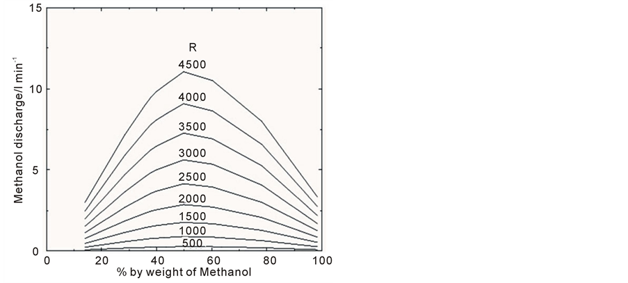
Figure 8. Methanol discharge rate DM required for a discharge with Froude number F = 14, plotted as a function of percentage weight of methanol PM (individual curves correspond to different Reynolds numbers).

Figure 9. Port diameter d required for a pure methanol discharge (PM = 100) with Froude number F = 14, plotted as a function of Reynolds number.
to 2.5% in 0.25% intervals, and from 2.5% up to 5.0% in 0.5% intervals. For each calibration measurement, an image was taken of a small transparent rectangular container filled with plume solution of a particular concentration, placed into the light sheet. The average greyscale pixel value over a selected area of the image was then determined.
A background image was also taken with the wave tank completely filled with dyed water. By removing this background image from images taken during the experiments, and also during the calibration measurements, imperfections in the light sheet could be compensated for.
Table 1 shows the parameters for each of the twelve experiments performed. Effluent was discharged from three different depths under a series of different wave amplitudes. By varying both the wave amplitude and discharge depth it was possible to produce a range of LQ/ZM values and investigate the effect of this on the dilution of the plume. For all experiments conducted with waves, the wavelength was 4.28 m.

Figure 10. Port discharge velocity uo required for a pure methanol discharge (PM = 100) with Froude number F = 14, plotted as a function of Reynolds number.

Figure 11. Total discharge rate DT required for a pure methanol discharge (PM = 100) with Froude number F = 14, plotted as a function of Reynolds number.

Table 1. Values of parameters for experiments performed. R = 4400, F = 14 and h/L = 0.16 for all experiments.
6. Results and Analyses
In order to compare the experimental results with theoretical values, instantaneous and time-averaged concentration maps were produced. For each of the twelve experiments performed, 50 of the captured greyscale CCD images (Figure 13 shows an example reverse video image as an illustration) were converted to instantaneous concentration maps. This was done by comparing the individual greyscale pixel values in each image with the greyscale pixel values for known concentrations of plume solution (established during the calibration measurements). The error in the instantaneous concentration measurements was estimated to be ±5% based on an analysis of the calibration procedure and measurement repeatability (so that, for example, a measured instantaneous concentration value of 1% could actually lie anywhere in the range 0.95% to 1.05%). Figure 14 shows a typical instantaneous concentration map of a plume. Meanwhile, for each experiment a time-averaged concentration map was determined by first averaging the individual greyscale pixel values across the 50 CCD images, and then comparing these averaged values with the greyscale pixel values for known concentrations of plume solu-

Figure 12. Wave tank equipped for LIF study of buoyant plumes.

Figure 13. Typical instantaneous reversed CCD image of the plume.
tion.
Figures 15-17 show time-averaged concentration maps for three of the twelve experiments carried out. From these images alone an increase in dilution due to the presence of waves can be seen. Figure 15 shows the situation with no waves present (LQ/ZM = 0), Figure 16 shows the discharge when small amplitude waves are present (LQ/ZM = 0.053) and Figure 17 shows the situation when the waves have a larger amplitude (LQ/ZM = 0.066). As LQ/ZM increases, the dilution of the plume has clearly also increased.
Analysis of each time-averaged concentration map with in-house software allows the centre line of the plume to be located and the change in concentration along that centre line to be found. Figure 18 shows the centre line concentrations (expressed as a percentage of the pure plume solution) plotted as a function of the normalized rise height (Z/H) for the time-averaged concentration maps of Figures 15-17. It can be seen that the “no waves” centre line concentration profile only follows the theoretical curve (derived from Equation (4)) in approximately the middle third of the rise height. The reason for this is that the theoretical curve is the solution for a line source and is therefore only valid once the individual plumes have merged, only then will the centre line concentration

Figure 14. Typical instantaneous concentration map of the plume.
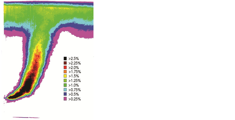
Figure 16. Concentration map for experiment 10 (see Table 1); small amplitude waves.
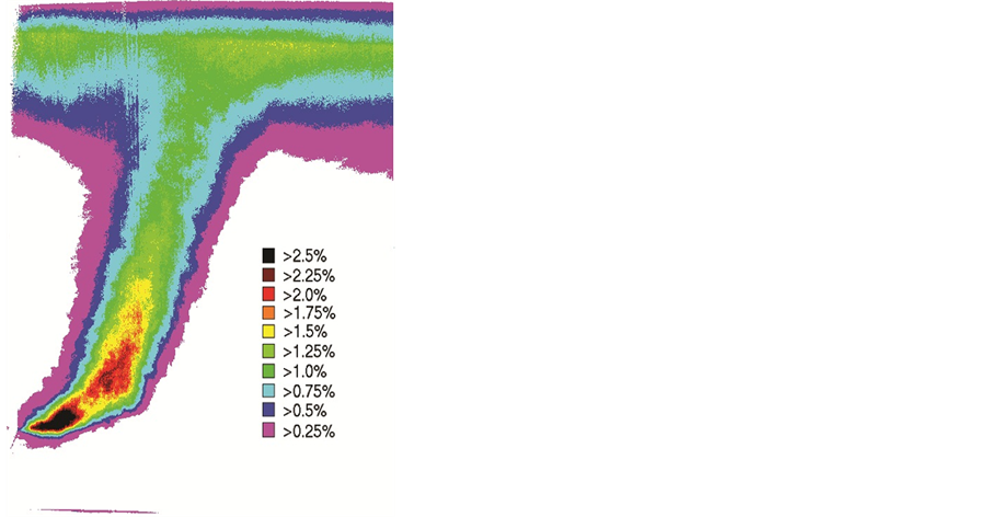
Figure 17. Concentration map for experiment 11 (see Table 1); large amplitude waves.
tend to the theoretical curve. Also, as can be seen from Figure 13, the final third of the rise height is through the effluent wastefield that forms at the surface. Within this region the analysis software was unable to accurately determine the position of the plume centre line and therefore the data will not be that for the true centre line.
The increased dilution due to the effect of the waves is again visible in Figure 18, with lower centre line concentrations observed when waves are present and with the greatest dilution occurring during the first fifth of the rise height. After this initial increase, dilution increases at a similar rate for both wave and no wave cases. This was observed by Chin [12] who noted the discharged jets “exploding” close to the port when the wave induced velocity opposed that of the discharge, but the plume merely being translated from side to side further above the port.
Chyan and Hwung [11] , although investigating a non-buoyant jet orientated vertically, also noted that the rise height could be divided into a number of regions. The first region (similar to Chin’s “exploding” region) they named the “deflection region”, as a vertical jet’s trajectory is deflected by the wave motion in this region. They also then identified a region of lower or decreased dilution as observed in the present results and noted that the increase in concentration was higher in stronger wave conditions. They named this the ‘transition region’ and argued that here the initial jet momentum had decayed to the extent that the jet flow was no longer significantly deflected. Indeed in the present results this increase in concentration takes place at around 2ZM in the rise height, the point at which the jet momentum becomes of the order of half the wave induced horizontal momentum. In this region the influence of the initial jet momentum has decreased to such an extent that it no longer influences the plume’s trajectory and motion is solely due to the wave effect. Above this point, as with the present results and with Chin’s results, they observed a “developed region” in which the plume is translated horizontally by the wave motion and identified by a decreased rate of dilution. The existence of these three different regions was confirmed by further experiments carried out by Mossa [5] on a vertical non-buoyant jet.
Koole and Swan [3] made related observations while investigating the effect of waves on a non-buoyant horizontal jet. In their work, they refer to a “zone of flow establishment” close to the jet source where the rate of dilution is high (analogous to Chin’s “exploding region”) and then a “zone of established flow” further away from the source where the dilution rate is substantially reduced. They suggest that wave motion promotes a transfer of momentum from the jet to the turbulent components of the flow field and that the effect is greatest within the “zone of flow establishment”. This leads to a significant increase in the turbulent Reynolds normal stresses in this region resulting in the high rate of dilution. Further evidence for this hypothesis is provided by Mossa [6] who also notes the contribution of the wave Reynolds normal stresses.
In order to quantify the effect of the waves on increasing plume dilution in the present work, a program was used to find the average increase in dilution in the region 0.1 < Z/H < 0.6 between wave and no wave cases (this region was chosen as this is the area in which the plume centre line detection program worked best). The increase in dilution can be expressed as S/So, where S is the centre line dilution with waves present and So is the centre line dilution under stagnant conditions. This increase S/So was then plotted against LQ/ZM (Figure 19). From the gradient of the line of best fit the increase in dilution due to the effect of the waves can be written as
 (18)
(18)
in good agreement with Chin’s equation [12] derived from measurements of dilution taken as the surface:
 (19)
(19)
The exploding effect observed by Chin also leads to a broadening of the plume as can be clearly seen by comparing Figures 15-17. This broadening can be quantified and further demonstrated as will now be shown.
First of all, additional analysis of each time-averaged concentration map using the in-house software enables the variation in concentration over the cross-section of the plume (i.e. normal to the centre line of the plume) to be determined at different heights above the diffuser. These cross-sectional concentration profiles are Gaussian in nature, as predicted by [1] . Therefore, by fitting a theoretical Gaussian curve to each cross-sectional concentration profile, it is possible to take 2 × the standard deviation corresponding to the fitted curve as being a measure of the plume width w at that particular height Z. For any given height, by subtracting the plume width when no waves are present from the plume width under the influence of surface waves (wn-w), the broadening of the plume due to the waves can be quantified. A non-dimensional parameter representing the broadening of the plume can be defined as , where aZ is the horizontal wave induced amplitude at height Z. Figure 20 and Figure 21, nondimensional plots of the broadening of the plume against rise height, show that the rate of broadening is increased for rise heights less than 2ZM, Chyan and Hwung’s deflection region. In this region the rate of broadening is 1.6 times higher than that for rise heights greater than 2ZM, with a line of best fit gradient of 1.1 × 10⁶ compared with a value of 0.69 × 10⁶ in the latter developed region.
7. Conclusions
Using an LIF technique it has been shown that, under wave conditions of the type present at the sites of outfalls,
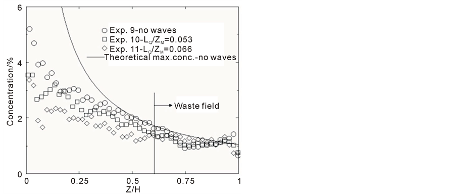
Figure 18. Plume centre line concentrations plotted as a function of normalized rise height.

Figure 19. Increase in centre line dilution of plume due to effect of waves plotted against LQ/ZM.
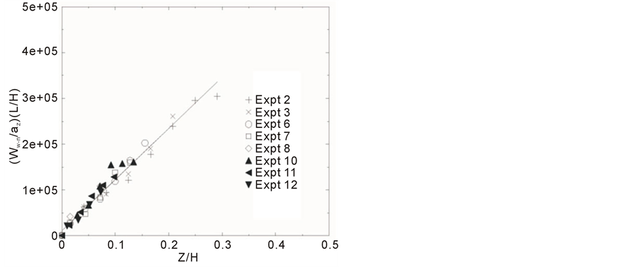
Figure 20. Non-dimensional plot of the broadening of the plume with increasing rise height (for Z < 2ZM).

Figure 21. Non-dimensional plot of the broadening of the plume with increasing rise height (for Z > 2ZM).
the dilution of a buoyant plume discharged from a multiport diffuser can be increased by wave effects. The full field nature of the technique has allowed not only the increase in dilution to be measured but also the region in which the enhanced mixing takes place to be clearly identified.
The average increase in dilution of the plume due to wave effects was found to be similar to the increase in surface dilution reported previously by other researchers. This is to be expected as the greatest increase in dilution was found to be in the region near to the diffuser and before individual plumes had merged. In this region, where the plume’s horizontal momentum is still greater than that of the wave induced motion, an “exploding” of the plume is seen. This results in an enhanced rate of broadening of the plume in this region. After this point, as the plume’s momentum decreases to half that of wave motion, the plume is merely oscillated by the wave motion and plume dilution is comparable to that of a plume released into quiescent conditions.
In future, a coupling of LIF and Particle Image Velocimetry techniques (such as demonstrated in [16] -[18] ) could be used to simultaneously produce instantaneous and time-averaged, full field concentration and velocity maps. This would allow a more complete study of the mechanics of a buoyant plume under the influence of surface waves.
Acknowledgements
This study was funded by the UK research councils EPSRC and NERC, whose support is gratefully acknowledged.
Nomenclature
a: wave amplitude.
aZ: horizontal wave induced amplitude at height Z above the diffuser.
B: buoyancy flux.
DT, DE and DM: total, ethanol and methanol discharge rates.
d: port diameter F: Froude number.
g and go: acceleration due to gravity and reduced gravity.
H: discharge depth.
h: total water depth.
k: wave number.
L: wavelength.
LM and LQ: length scales.
M: momentum flux.
PE and PM: percentages by weight of ethanol and methanol.
Q: volume flux.
R: Reynolds number.
S and So: centreline dilution with and without waves.
Sm: minimum centreline dilution.
s: port spacing.
T: wave period.
uo: port discharge velocity.
umax: maximum horizontal wave induced velocity at port.
w: plume width (2 × standard deviation associated with the fitted theoretical Gaussian curve).
wn-w: plume width under influence of waves-plume width when no waves present.
Z: height measured vertically from diffuser.
ZM: rise height for plume momentum to be of the order of the wave induced momentum.
μo: initial viscosity of discharge.
νo: kinematic viscosity of discharge.
ρo and ρa: initial density of discharge and ambient fluid.
σ: wave frequency.